Interest points
Interest points. CSE P 576 Larry Zitnick ( larryz@microsoft.com ) Many slides courtesy of Steve Seitz. How can we find corresponding points?. Not always easy. NASA Mars Rover images. Answer below (look for tiny colored squares…). NASA Mars Rover images


Interest points
E N D
Presentation Transcript
Interest points CSE P 576 Larry Zitnick (larryz@microsoft.com) Many slides courtesy of Steve Seitz
Not always easy NASA Mars Rover images
Answer below (look for tiny colored squares…) NASA Mars Rover images with SIFT feature matchesFigure by Noah Snavely
Where do humans fixate? Called “fixation points”, and a “saccade” is the process of moving between fixation points. Slowly trace the outline of the above object.
Where do humans fixate? Called “fixation points”, and a “saccade” is the process of moving between fixation points. Slowly trace the outline of the above object.
Where do humans fixate? Result of one subject “me”.
Where do humans fixate? Top down or bottom up? "Eye Movements and Vision" by A. L. Yarbus; Plenum Press, New York; 1967
Want uniqueness Look for image regions that are unusual • Lead to unambiguous matches in other images How to define “unusual”?
Local measures of uniqueness Suppose we only consider a small window of pixels • What defines whether a feature is a good or bad candidate? Slide adapted from Darya Frolova, Denis Simakov, Weizmann Institute.
Feature detection Local measure of feature uniqueness • How does the window change when you shift by a small amount? “corner”:significant change in all directions “flat” region:no change in all directions “edge”: no change along the edge direction Slide adapted from Darya Frolova, Denis Simakov, Weizmann Institute.
Principle Component Analysis How to compute PCA components: Subtract off the mean for each data point. Compute the covariance matrix. Compute eigenvectors and eigenvalues. The components are the eigenvectors ranked by the eigenvalues. Principal component is the direction of highest variance. Next, highest component is the direction with highest variance orthogonal to the previous components. Both eigenvalues are large!
Simple example Detect peaks and threshold to find corners.
The math To compute the eigenvalues: Compute the covariance matrix. Compute eigenvalues. Typically Gaussian weights
The Harris operator • - is a variant of the “Harris operator” for feature detection • Very similar to - but less expensive (no square root) • Called the “Harris Corner Detector” or “Harris Operator” • Lots of other detectors, this is one of the most popular Actually used in original paper:
The Harris operator Harris operator
How can we find correspondences? Similarity transform
Scale and rotation? Let’s look at scale first: What is the “best” scale?
Scale The Laplacian has a maximal response when the difference between the “inside” and “outside” of the filter is greatest.
Scale Why Gaussian? It is invariant to scale change, i.e., and has several other nice properties. Lindeberg, 1994 In practice, the Laplacian is approximated using a Difference of Gaussian (DoG).
DoG example σ = 1 σ = 66
Scale In practice the image is downsampled for larger sigmas. Lowe, 2004.
How to compute the rotation? Rotation Create edge orientation histogram and find peak.
Harris Laplace Other interest point detectors Scale & Affine Invariant Interest Point Detectors K. MIKOLAJCZYK and C. SCHMID, IJCV 2004
Affine invariant Other interest point detectors Scale & Affine Invariant Interest Point Detectors K. MIKOLAJCZYK and C. SCHMID, IJCV 2004
Computationally efficient Approximate Gaussian filters using box filters: SURF: Speeded Up Robust Features Herbert Bay, TinneTuytelaars, and Luc Van Gool, ECCV 2006
Corner detection by sampling pixels based on decision tree Computationally efficient Machine learning for high-speed corner detection Edward Rosten and Tom Drummond, ECCV 2006
Let’s go to the videos… How well do they work in practice?