
Routing Algorithms in Internet Networking
E N D
Presentation Transcript
Routing: Link State Algorithm Networking CS 3470, Section 1
Routing • Forwarding versus Routing • Forwarding: • To select an output port based on destination address and routing table • Routing: • Process by which routing table is built
Forwarding Table vs Routing Table • Forwarding table • Used when a packet is being forwarded • Must contain enough information to forward • A row in the forwarding table contains • Mapping from a network number to outgoing interface • MAC or Ethernet address of the next hop
Forwarding Table vs Routing Table • Routing table • Built by the routing algorithm as a precursor to build the forwarding table • Generally contains mapping from network numbers to next hops
Routing • An autonomous system (AS) is a network that is administrated independently of other ASs • Backbone service providers and regional providers form their own ASs • Can run their own (different) routing algorithms • Also called routing domains
NAP National Provider NAP NAP NAP National Provider Regional Provider customers NAPs, NSPs, ISPs • NSP: National Service Provider (Tier 1 Providers/Backbones) • Example: CenturyLink, Telia Carrier, NTT, Cogent, Level 3, GTT, and Tata Communications. • NAP: Network Access Point
MAE-West Exchange Point Pacific Bell Exchange Point Ameritech Exchange Point Sprint Exchange Point MAE-East Exchange Point Private Peering Private Peering Private Peering Private Peering Private Peering Private Peering Private Peering Private Peering InternetNetwork Example of a National Service Provider (Sprint)
C.b B.a A.a c A.c b a c b Intra-AS and Inter-AS Routing • Gateways: • perform inter-AS routing amongst themselves • perform intra-AS routers with other routers in their AS b a a C B d A
C.b B.a A.a c A.c b a c b Intra-AS and Inter-AS Routing • Gateways: • perform inter-AS routing amongst themselves • perform intra-AS routers with other routers in their AS b a a C B d A network layer inter-AS, intra-AS routing in gateway A.c link layer physical layer
Inter-AS routing between A and B C.b B.a A.a b c A.c a a C b B a Host h1 d c b A • We’ll now examine both inter-AS and intra-AS Internet routing protocols Intra-AS and Inter-AS Routing Host h2 Intra-AS routing within AS B Intra-AS routing within AS A
Intra-AS Routing • a.k.a., “routing in the small” • These routing algorithms only scale for smaller networks (few hundred nodes), but set the stage for the hierarchical Inter-AS routing protocols used in the Internet today
B C A F E D Routing Network as a Graph • The basic problem of routing is to find the lowest-cost path between any two nodes • Where the cost of a path equals the sum of the costs of all the edges that make up the path 5 3 5 2 2 1 3 1 2 1
Routing • For a simple network, we can calculate all shortest paths and load them into some nonvolatile storage on each node. • Such a static approach has several shortcomings • It does not deal with node or link failures • It does not consider the addition of new nodes or links • It implies that edge costs cannot change
Routing • Instead of a static approach, we need a dynamic way to find the lowest-cost path • Node and link failures, changing link costs • We would like these algorithms to be distributed so that they can be somewhat scalable
Distributed Routing Algorithms • Routers cooperate using a distributed protocol • To create mutually consistent routing tables • Two standard distributed routing algorithms • Link state routing • Distance vector routing
Link State vs Distance Vector • Both assume that • The address of each neighbor is known • The costof reaching each neighbor is known • Both find global information • By exchanging routing info among neighbors • Differ in info exchanged and route computation • LS: tells every other node its distance to neighbors • DV: tells neighbors its distance to every other node
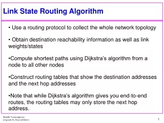
Link State Algorithm • Basic idea: Distribute to all routers • Cost of each link in the network • Each router independently computes optimal paths • From itself to every destination • Routes are guaranteed to be loop free if • Each router sees the same cost for each link • Uses the same algorithm to compute the best path
Topology Dissemination • Each router creates a set of link state packets (LSPs) • Describing its links to neighbors • LSP contains • Router id, neighbor’s id, and cost to its neighbor • Copies of LSPs are distributed to all routers • Using controlled flooding • Each router maintains a topology database • Database containing all LSPs
Dijkstra’s Algorithm • Given the network topology • How to compute shortest path to each destination? • Some notation • X: source node • N: set of nodes to which shortest paths are known so far • N is initially empty • D(V): cost of known shortest path from source X from V • C(U,V): cost of link U to V • C(U,V) = if not neighbors
Algorithm (at Node X) • Initialization • N = {X} • For all nodes V • If V adjacent to X, D(V) = C(X,V) else D(V) = • Loop • Find U not in N such that D(U) is smallest • Add U into set N • Update D(V) for all V not in N • D(V) = min{D(V), D(U) + C(U,V)} • Until all nodes in N
B C A F E D Let’s take a look at an example • Sample network 5 3 5 2 2 1 3 1 2 1
B C A F E D Link State Database • Starting global database • Each router has it’s own starting link state database 5 3 5 2 2 1 3 1 2 1
B C A F E D Dijkstra’s Algorithm: Initialization for Node A D(B),p(B) 2,A D(D),p(D) 1,A D(C),p(C) 5,A D(E),p(E) infinity Step 0 1 2 3 4 start N A D(F),p(F) infinity D(x) is distance/cost to x p(x) is path to x 5 3 5 2 2 1 3 1 2 1
B C A F D E Dijkstra’s algorithm: example D(B),p(B) 2,A 2,A D(D),p(D) 1,A D(C),p(C) 5,A 4,D D(E),p(E) infinity 2,D Step 0 1 2 3 4 start N A AD D(F),p(F) infinity infinity Now we select the node with the shortest distance to add to set N. Then we update distances of other nodes if they can be made shorter going through D. 5 3 5 2 2 1 3 1 2 1
B C A F D E Dijkstra’s algorithm: example D(B),p(B) 2,A 2,A D(D),p(D) 1,A D(C),p(C) 5,A 4,D 4,D D(E),p(E) infinity 2,D 2,D Step 0 1 2 3 4 start N A AD ADB D(F),p(F) infinity infinity infinity B has the next shortest distance from A, so we add it to set N. (could have been E..) Then we update distances of other nodes if they can be made shorter going through B… 5 3 5 2 2 1 3 1 2 1
B C A F D E Dijkstra’s algorithm: example D(B),p(B) 2,A 2,A D(D),p(D) 1,A D(C),p(C) 5,A 4,D 4,D 3,E D(E),p(E) infinity 2,D 2,D Step 0 1 2 3 4 start N A AD ADB ADBE D(F),p(F) infinity infinity infinity 4,E 5 3 5 2 2 1 3 1 2 1
B C A F D E Dijkstra’s algorithm: example D(B),p(B) 2,A 2,A 2,A D(D),p(D) 1,A D(C),p(C) 5,A 4,D 4,D 3,E D(E),p(E) infinity 2,D 2,D Step 0 1 2 3 4 start N A AD ADB ADBE ADBEC D(F),p(F) infinity infinity infinity 4,E 4,E 5 3 5 2 2 1 3 1 2 1
B C A F D E Dijkstra’s algorithm: example D(B),p(B) 2,A 2,A 2,A D(D),p(D) 1,A D(C),p(C) 5,A 4,D 4,D 3,E D(E),p(E) infinity 2,D 2,D Step 0 1 2 3 4 5 start N A AD ADB ADBE ADBEC ADBECF D(F),p(F) infinity infinity infinity 4,E 4,E This process terminates after all the nodes are added to N. 5 3 5 2 2 1 3 1 2 1
B C A F D E Routing Table Computation • Now we know how to construct a shortest paths spanning tree. • How do we get the routing table from this tree? • Routing table is essentially a mapping from destination to next hop. 5 3 5 2 2 1 3 1 2 1
A A A A D B D D B B D B C C C C Dijkstra’s algorithm, discussion • Oscillations possible: • e.g., link cost = amount of carried traffic 1 1+e 2+e 0 2+e 0 2+e 0 0 0 1 1+e 0 0 1 1+e e 0 0 0 e 1 1+e 0 1 1 e … recompute … recompute routing … recompute initially