Understanding Link State Routing in Computer Networking
220 likes | 315 Views
Explore Link State Routing, a routing algorithm where routers share network topology information to compute optimal paths. Learn about the phases of flooding and Dijkstra's algorithm, complexities of OSPF, message complexity, and choosing between Link State and Distance Vector protocols. Gain insights into cost metrics and challenges in handling network failures and scalability.

Understanding Link State Routing in Computer Networking
E N D
Presentation Transcript
Link State Routing • Same assumptions/goals, but different idea than DV: • Tell all routers the topology and have each compute best paths • Two phases: • Topology dissemination (flooding) • New News travels fast. • Old News should eventually be forgotten • Shortest-path calculation (Dijkstra’s algorithm) - nlogn
Flooding • Each router maintains link state database and periodically sends link state packets (LSPs) to neighbor • LSPs contain [router, neighbors, costs] • Each router forwards LSPs not already in its database on all ports except where received • Each LSP will travel over the same link at most once in each direction • Flooding is fast, and can be made reliable with acknowledgments
Example • LSP generated by X at T=0 X A X A T=0 T=1 C B D C B D X A X A T=2 T=3 C B D C B D
Complications • When link/router fails need to remove old data. How? • LSPs carry sequence numbers to determine new data • Send a new LSP with cost infinity to signal a link down • What happens if the network is partitioned and heals? • Different LS databases must be synchronized
Shortest Paths: Dijkstra’s Algorithm • N: Set of all nodes • M: Set of nodes for which we think we have a shortest path • s: The node executing the algorithm • L(i,j): cost of edge (i,j) (inf if no edge connects) • C(i): Cost of the path from s to i. • Two phases: • Initialize C(n) according to received link states • Compute shortest path to all nodes from s • Link costs are symmetric
The Algorithm // Initialization M = {s} // M is the set of all nodes considered so far. For each n in N - {s} C(n) = L(s,n) // Find Shortest paths Forever { Unconsidered = N-M If Unconsidered == {} break M = M + {w} such that C(w) is the smallest in Unconsidered For each n in Unconsidered C(n) = MIN(C(n), C(w) + L(w,n)) }
Open Shortest Path First (OSPF) • Most widely-used Link State protocol today • Basic link state algorithms plus many features: • Authentication of routing messages • Extra hierarchy: partition into routing areas • Only bordering routers send link state information to another area • Reduces chatter. • Border router “summarizes” network costs within an area by making it appear as though it is directly connected to all interior routers • Load balancing
Distance Vector Message Complexity N: number of nodes in the system M: number of links D: diameter of network (longest shortest path) • Size of each update: • Number of updates sent in one iteration: • Number of iterations for convergence: • Total message cost: • Number of messages: • Incremental cost per iteration:
Link State Message Complexity • Each link state update size: d(i) where d(i) is degree of node i • Number of messages per broadcast: • Bytes per link state update broadcast: • Total messages across all link state updates: • Total bytes across all link state updates:
Distance Vector vs. Link State • When would you choose one over the other?
Why have two protocols? • DV: “Tell your neighbors about the world.” • Easy to get confused • Simple but limited, costly and slow • Number of hops might be limited • Periodic broadcasts of large tables • Slow convergence due to ripples and hold down • LS: “Tell the world about your neighbors.” • Harder to get confused • More expensive sometimes • As many hops as you want • Faster convergence (instantaneous update of link state changes) • Able to impose global policies in a globally consistent way • load balancing
Cost Metrics • How should we choose cost? • To get high bandwidth, low delay or low loss? • Do they depend on the load? • Static Metrics • Hopcount is easy but treats OC3 (155 Mbps) and T1 (1.5 Mbps) • Can tweak result with manually assigned costs • Dynamic Metrics • Depend on load; try to avoid hotspots (congestion) • But can lead to oscillations (damping needed)
Revised ARPANET Cost Metric • Based on load and link • Variation limited (3:1) and change damped • Capacity dominates at low load; we only try to move traffic if high load 225 140 New metric (routing units) 90 75 60 30 9.6-Kbps satellite link 9.6-Kbps terrestrial link 25% 50% 75% 100% 56-Kbps satellite link Utilization 56-Kbps terrestrial link
Key Concepts • Routing uses global knowledge; forwarding is local • Many different algorithms address the routing problem • We have looked at two classes: DV (RIP) and LS (OSPF) • Challenges: • Handling failures/changes • Defining “best” paths • Scaling to millions of users
Dijkstra Example – After the flood * * 1 10 2 3 9 0 4 6 7 5 2 The Unconsidered. The Considered
1 10 inf 10 2 3 9 0 4 6 7 5 inf 5 2 Dijkstra Example – Post Initialization * * The Unconsidered. The Considered
The Considered The Unconsidered. The Under Consideration (w). Considering a Node 1 10 inf 10 2 3 9 0 4 6 7 5 inf 5 2 Cost updates of 8,14, and 7
The Considered The Unconsidered. The Under Consideration (w). Pushing out the horizon 1 8 14 2 3 9 0 4 6 7 5 7 5 2 Cost updates of 13
The Considered The Unconsidered. The Under Consideration (w). Next Phase 1 8 13 2 3 9 0 4 6 7 5 7 5 2 Cost updates of 9
The Considered The Unconsidered. The Under Consideration (w). Considering the last node 1 8 9 2 3 9 0 4 6 7 5 7 5 2
Dijkstra Example – Done 1 8 9 2 3 9 0 4 6 7 5 7 5 2