Sampling Distribution of Sample Means

1. Sampling Distribution of a Sample Mean Lecture 28 Section 8.4 Mon, Mar 20, 2006

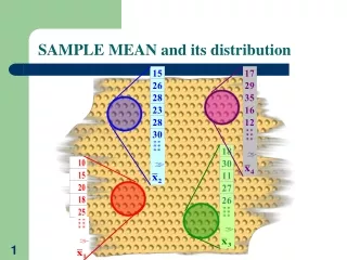
2. Sampling Distribution of the Sample Mean • Sampling Distribution of the Sample Mean– The distribution of sample means over all possible samples of the size n from that population.

3. With or Without Replacement? • If the sample size is small in relation to the population size (< 5%), then it does not matter whether we sample with or without replacement. • The calculations are simpler if we sample with replacement. • In any case, we are not going to worry about it.

4. Example • Suppose a population consists of the numbers {1, 2, 3}. • Using samples of size n = 1, 2, or 3, find the sampling distribution ofx. • Draw a tree diagram showing all possibilities.

5. The Tree Diagram • n = 1 mean = 1 1 mean = 2 2 mean = 3 3

6. The Sampling Distribution • The sampling distribution ofx is • The parameters are •  = 2 • 2 = 2/3 = 0.6667

7. The Tree Diagram mean 1 1 2 1 1.5 2 3 1 1.5 2 2 2 2.5 3 1 2 3 2 2.5 3 3

8. The Sampling Distribution • The sampling distribution ofx is • The parameters are •  = 2 • 2 = 2/6 = 0.3333

9. The Tree Diagram 1 1 1 2 4/3 3 5/3 1 4/3 2 1 2 5/3 3 2 1 5/3 2 2 3 7/3 3 1 4/3 1 2 5/3 3 2 1 5/3 2 2 2 2 3 7/3 1 2 3 2 7/3 3 8/3 1 5/3 1 2 2 3 7/3 3 1 2 2 2 7/3 3 8/3 1 7/3 3 2 8/3 3 3

10. The Sampling Distribution • The sampling distribution ofx is • The parameters are •  = 2 • 2 = 2/9 = 0.2222

11. Sampling Distributions • Run the program Central Limit Theorem for Means.exe. • Use n = 30 and population = {1, 2, 3}; generate 100 samples.

12. 100 Samples of Size n = 30  = 0.75  = 0.079

13. Observations and Conclusions • Observation #1: The values ofx are clustered around . • Conclusion #1:x is probably close to .

14. Larger Sample Size • Now we will select 100 samples of size 120 instead of size 30. • Run the program Central Limit Theorem for Means.exe. • Pay attention to the spread (standard deviation) of the distribution.

15. 100 Samples of Size n = 120  = 0.75  = 0.0395

16. Observations and Conclusions • Observation #2: As the sample size increases, the clustering is tighter. • Conclusion #2A: Larger samples give more reliable estimates. • Conclusion #2B: For sample sizes that are large enough, we can make very good estimates of the value of .

17. Larger Sample Size • Now we will select 10000 samples of size 120 instead of only 100 samples. • Run the program Central Limit Theorem for Means.exe. • Pay attention to the shape of the distribution.

18. 10,000 Samples of Size n = 120  = 0.75  = 0.0395

19. 10,000 Samples of Size n = 120

20. More Observations and Conclusions • Observation #3: The distribution ofx appears to be approximately normal.

21. One More Conclusion • Conclusion #3: We can use the normal distribution to calculate just how close to  we can expectx to be. • However, we must know the values of  and  for the distribution ofx. • That is, we have to quantify the sampling distribution ofx.

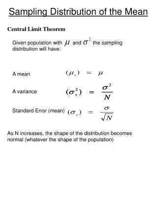
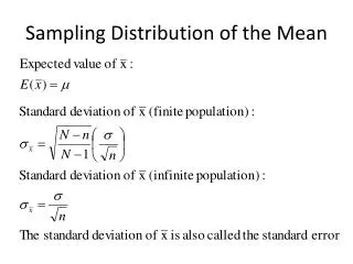
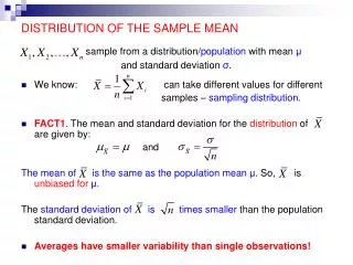
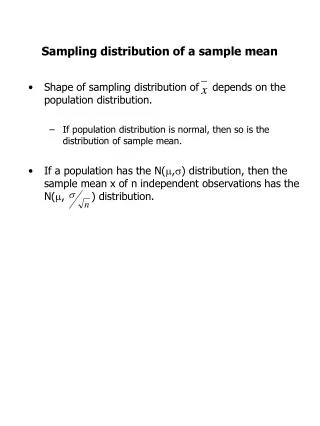
22. The Central Limit Theorem • Begin with a population that has mean  and standard deviation . • For sample size n, the sampling distribution of the sample mean is approximately normal with

23. The Central Limit Theorem • The approximation gets better and better as the sample size gets larger and larger. • That is, the sampling distribution “morphs” from the distribution of the original population to the normal distribution. • For many populations, the distribution is almost exactly normal when n  10. • For almost all populations, if n 30, then the distribution is almost exactly normal.

24. The Central Limit Theorem • Therefore, if the original population is exactly normal, then the sampling distribution of the sample mean is exactly normal for any sample size. • This is all summarized on pages 536 – 537.

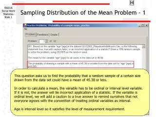
25. Example • Based on past data, a student’s average score on individual homework problems is 7.3 points out of 10, with a standard deviation of about 2.9 points. • This counts only those homework problems that were attempted.

26. Example • Over the course of the semester, I sample (grade) approximately 100 homework problems per student. • Thus, n = 100. • What is the sampling distribution of the homework average (for the typical student)?

27. Example • Based on the Central Limit Theorem for Means, the sampling distribution • Is normally distributed (n  30) • Has a mean of 7.3 points. • Has a standard deviation of 2.9/100 = 0.29 points. • On a 100-point scale, that would be • An average of 73. • A standard deviation 2.9.

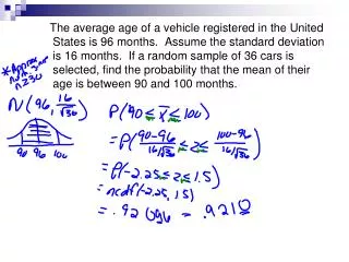
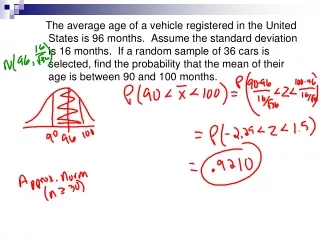
28. Example • What is the probability that a student’s homework average (100 sampled problems) will be within 5 points of his true average for all problems?

29. Example • For the typical student, that would be a homework average between 68 and 78. • normalcdf(68, 78, 73, 2.9) = 0.9153, or about 92%

30. Point of Fact • Since the sample size (n = 100) is a sizable fraction of the population size (N = 400) and we are sampling without replacement, we should take into account the “finite population correction factor” of (N – n)/(N – 1) for the variance ofx.

31. Point of Fact • For n = 100 and N = 400, this factor is 0.8671. • Thus, in fact, the typical standard deviation is only about 0.251, or 2.51 points out of 100. • Recompute: normalcdf(68, 78, 73, 2.51) = 0.9536, or 95.36%.