Download
1 / 28
280 likes | 531 Views
CORRELATON & REGRESSION. C orrelation and regression are concerned with the investigation of relationships between two or more variables. We consider just two associated variables. We might want to know: If a relationship exists between those variables

E N D
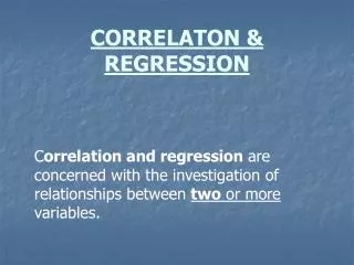
CORRELATON & REGRESSION Correlation and regression are concerned with the investigation of relationships between two or more variables.
We consider just two associated variables. We might want to know: • If a relationship exists between those variables • If so, how strong that relationship is • What form that relationship takes • Can we make use of that relationship for predictive purposes i.e. forecasting?
Correlation is used to find the strength of the relationship Regression describes the relationship itself in the form of an equation which best fits the data General method for investigating the relationship between 2 variables:
For an initial insight into the relationship between two variables: • plot a scatter diagram • If there appears to be a linear relationship, quantify it: • calculate the correlation coefficient This is a measure of the strength of this linear relationship. Its symbol is 'r' and its value lies between -1 and +1
If the relationship is found to be significantly strong: • find the equation of the ‘line of best fit’ through the data, using linear regression • The 'goodness of fit'statisticcan be calculated to see how useful the regression equation is likely to be • Once defined by an equation, the relationship can be used for predictive purposes.
Example The data represents a sample of advertising expenditures and sales for ten randomly selected months. See slide 12 for complete data. MonthAdvertisingSales expenditure(£0.000’s) y (£0,000’s) x 1 1.2 101 2 0.8 92 3 1.0 110 etc. Plot a scatter diagram of the data
Note scales are not started at zero The graph suggests a linear relationship between sales and advertising expenditure. The larger the amount spent on advertising the higher the sales in general.
If there is a relationship, we need to be able to measure the strength of that relationship. i.e. calculate the value of the correlation coefficient
Pearson's Product Moment Correlation Coefficient (r) is a measure of how close a linear relationship there is between x and y. can be produced directly from a calculator in LR (linear regression) mode For the sales and advertising data the correlation coefficient: r = 0.875 The value of r is always between + 1 and -1
r = -1 perfect negative correlation r = -0.7 r = 0 no correlation r = +0.8 r = +1 perfect positive correlation
Formula for correlation coefficient, r r = Sxy Sxx Syy where Sxx = Sx2 - Sx Sx n Syy = Sy2 - Sy Sy n Sxy = Sx2 - Sx Sy n
Step 1 Longhand calculations for correlation coefficient r.
Step 2 Therefore: Sxx = Sx2 - Sx Sx = 9.28 - 9.4 x 9.4 = 0.444 n 10 Syy = Sy2 - Sy Sy = 93569 - 959 x 959 = 1600.9 n 10 Sxy = Sxy - Sx Sy = 924.8 - 9.4 x 959= 23.34 n 10 Step 3 Therefore: r = Sxy = 23.34 = 0.875 Sxx Syy 0.444 x 1600.9
Hypothesis test for the value of r We shall not go into the details here! Null hypothesis (H0): A linear relationship does not exist between sales and advertising Alternative hypothesis(H1): A linear relationship does exist between sales and advertising. If we calculate a test statistic and critical value we discover that test statistic > critical value so we reject H0 Conclude that a linear relationship exists between sales and amount spent on advertising.
The Goodness of Fit Statistic (R2) This also measures of the closeness of the relationship between x and y R2 = 100r2 R2 tells us what percentage of the total variation in y (here sales) is explained by the variation in x (here advertising expenditure)
Interpretation: • If r = +1 or –1, then R2 =100% So 100% of the variation in y is explained by the variation in x. • If r = 0, then R2 = 0% So none of the variation in y is explained by the variation in x • For the data above the goodness of fit statistic R2 = 100 r2 = 100 x 0.8752 = 76.6%
76.6% of the variation in sales is explained by the variation in the amount spent on advertising. The remaining 23.4% of the variation is explained by other factors: e.g. price competitor’s prices etc.
Regression equation Since we know, for the sample data, that there is a significant relationship between the two variables, the next obvious step is to find its equation. We can then add the regression line to the scatter diagram and use it to predict future sales, given advertising expenditure for a particular month. The regression equation can be produced directly from a calculator in LR mode.
Theregression line has the equation: y = a + bx x is the independent variable y is the dependent variable a is the intercept on the y-axis b is the gradient or slope of the line.
For the sales and advertising data, the values of a and b are 46.5 and 52.6. So regression equation is: y = 46.5 + 52.6x Sales = 46.5 + 52.6 advertising (a and b can be found using LR mode on your calculator or by calculation)
Formula for a and b This is found by calculating the square ofthe differences between actual and expected values. We chose a and b so that the total difference is minimizied: b = Sxy a = y - b x Sxx ( x , y ) is called the centroid Where x , y are the meansof the x and y data and the S’s are defined as previously.
Calculations for the regression equation. In the regression equation y = a + bx b = Sxy = 23.34 = 52.6 Sxx 0.444 a = y - b x = 95.9 - 52.6 x 0.94 = 46.5 (Asy = Sy = 959 and x = Sx = 9.4 = 0.94) n 10 n 10 Therefore the regression equation is y = 46.5 + 52.6x
Plotting the regression equation on the scatter diagram. The line y = a + bx can be plotted on the scatter diagram by plotting three points. The centroid ( x , y ) and any other two points, which satisfy the regression equation. From the data (x, y) = (0.94, 95.9) When x = 0.6, y = 46.5 + (52.6 x 0.6) = 78.06 When x = 1.2, y = 46.5 + (52.6 x 1.2) = 109.6 Plot (0.94,95.9) Plot (0.6, 78.6) Plot (1.3, 109.6)
x x x x
Note • regression equation y = a + bx can only be used to calculate an estimate for y given the value of x • The linear relationship y = a + bx can only be assumed to exist between y and x for the range of values within the sample
Interpreting the coefficients in the regression equation - first the a value The intercept (a) is the estimate of y when x = 0, but care is needed if using this – why? y = 46.5 + 52.6x Sales = 46.5 + 52.6 advertising When x = 0, y = 46.5 i.e. When nothing is spent on advertising, sales would be expected on average to be 46.5 units = 46.5 x £10,0000 =£ 465,000
the b value y = 46.5 + 52.6x If x = 0 y = 46.5, but care is needed here! If x = 0.6 y = 46.5 + (52.6)(0.6) = If x = 0.8 y = 46.5 + (52.6)(0.8) = If x = 1 y = 46.5 + 52.6 = If x = 1.2 y = 46.5 + (52.6)(1. 2) = If x = 2 y = 46.5 + 52.6 x 2 but care is needed here also! etc. So if advertising expenditure is increased by 1 unit, sales will be increased by 52.6 units on average.
For each additional £10,000 spent on advertising, sales will increase by £52.6 x £10,000 = £526,000 on average. But we cannot estimate sales outside the range: E.g. we should not try to estimate sales for x = 5 using this method.