SPSS 202: Linear and Logistic Regression Using SPSS (Workshop)
800 likes | 2.04k Views
SPSS 202: Linear and Logistic Regression Using SPSS (Workshop) . Dr. Daisy Dai Department of Medical Research. Contents. Correlation (Pearson, Spearman, r-square) Scatter Plot and Trending Simple regression Multiple regression Logistic regression . Introduction to SPSS. What is SPSS?.

SPSS 202: Linear and Logistic Regression Using SPSS (Workshop)
E N D
Presentation Transcript
SPSS 202: Linear and Logistic Regression Using SPSS (Workshop) Dr. Daisy Dai Department of Medical Research
Contents • Correlation (Pearson, Spearman, r-square) • Scatter Plot and Trending • Simple regression • Multiple regression • Logistic regression
What is SPSS? • Statistical software. • CMH has 10 server licenses. • SPSS 18.
SPSS Data Entry • SPSS data can be entered manually. • The format is ready for analysis. • SAS, Excel, txt, etc. data can be easily imported to SPSS. • SPSS data files are saved as “SPSS data document (.sav)”. • SPSS output files are saved as “SPSS viewer document (.spv)”.
SPSS Data Entry • SPSS has a few unique features in data entry. • Categorical variables need to be coded. For instance, code male as 1 and female as 0 or vice versa. • When you have two treatments, test and control, please use 1 for test and 0 for control. • Categorical variables that are not coded in other sourced data files will not be imported or analyzed properly in SPSS. • Continuous variables don’t need coding. • Missing values needs to be defined in “variable view” page.
Log in SPSS • CMH offers server version SPSS 18. Any employee can log in SPSS from your employee account. • Go to Start ->Program ->Accessories -> Remote Desktop Connection
Log in SPSS • In the prompted connection window, enter cmhterm. • ClickConnect.
Log in SPSS • In the Log On Window, enter your cmh user name and password. • Choose log on to CMH • ClickOK.
Data Set 1: Anemia in Women • A survey was conduct to a sample of 20 anemia women, randomly selected from a pre-defined geographical area. The participants had a blood sample taken and their hemoglobin (Hb) level and packed cell volume (PCV) measured. They were also asked their age, and whether or not they had experienced the menopause. • The goals of the study were to determine whether Hb affects PCV or the other way around or whether Hb was associated with age.
Tasks • Import data • View and modify data • Scatter plot and trending • Save the results.
Task 1: Import Data • Double click spss 18 icon on the screen. • Click File -> Open -> Data. • Click OK.
Task 1: Import Anemia Data • Select the folder where data saved. (Note: since SPSS is in the server, we need to save files in the net work drive. I usually save files to my account in U drive. ) • Enter file name. • Select file type. (SPSS data file is in .sav format. SPSS can open excel or many other files, please make sure you choose the right file type). • Click Open.
Task 2: View and Modify Data • Now the data is open. • There are two tabs on the screen, data view tab and variable view tab. • We can read the data in “data View” tab.
Task 2: View and Modify Data • We can define data structure including variable name, label, etc. in “Variable View” tab. • Note the categorical variable, menopause, needs to be coded in the values column. Enter 0 for No and 1 for Yes.
Task 3: Scatter Plot • Generate scatter plot between Hb and PCV. • Please list the dependent (outcome) variable in y-axis and the independent (explanatory) variable in x-axis.
Task 3: Scatter Plot • Click Graphs -> Legacy Dialogs -> Scatter/Dot -> Simple Scatter -> Define
Task 3: Scatter Plot • All variables in the Anemia data set is listed in the left panel • Select the variables for y axis and x-axis by first clicking the variable in the left panel and then clicking the arrow and the corresponding spot in the right panel. • The marker variable is optional. If you want to label the subjects, then choose the corresponding variable as the marker. For instance, you can label the subjects by ID or by menopause. Here we choose menopause. • Click OK.
Task 3: Scatter Plot • One can double click the figure to prompt Chart Editor. • Click on the fitted line icon located in the middle of last line of tool bar. • We can also edit font or add in text box. • Close Chart Editor.
Task 3: Scatter Plot • One can fit linear, quadratic or cubic trend along with confidence interval to the data. • Loess (local regression) is an useful tool to fit non-linear and irregular data.
Task 4: Save output • One can save SPSS output file by clicking file -> save as to generate a viewer file in. apv format. This file can be edited by SPSS in the future. • Or one can export the figure by right click and export to a word or pdf document. This file is permanent without revision to figures.
Practice • Generate scatter plot between Hb and age. • Fit an appropriate trend. • Use Chart Editor to edit the font and add text when needed. • Save the figure. • Interpret the scatter plot and r-square.
Tasks • Continue with anemia data. • Determine Pearson and Spearman correlation among the continuous variables • Interpret results
Correlation • On the data page, click Analyze-> Correlat-> Bivariate
Correlation • We have three continuous variables in the data sets: Hb, PCV and Age. • Select these three variables and check Pearson (parametric) and Spearman (non-parametric). • Check two-tailed for conservative analysis • And flag significant correlations. • Click OK.
Pearson and Spearman Correlation Nonparametric correlations are based on ranks of data and it can be applied when data does not follow normality assumption (skewed) or outlier exists.
Tasks • Continue using anemia data. • Perform simple linear regression. • Determine the fitted regression model.
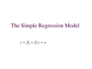
Simple Regression • Click Analyze-> Regression -> Linear
Regression • Select Hb as Dependent variable (y axis). • Select PCV as Independent variable (x axis). • In this case, PCV is the explanatory variable and Hb is the outcome variable. In other words, we investigate how PCV will impact Hb. • Click Ok.
Hb=5.589+0.205*PCV When PCV=35, the predicted Hb=5.589+0.205*35=12.8 PCV is significantly associated with Hb with p-value=0.001
Tasks • Continue with anemia data. • Consider PCV and age as two risk factors associated with Hb.
Multiple Regression • Click Analyze-> Regression -> Linear
Multiple Regression • Select Hb as Dependent variable. • Select PCV and age as Independent variable. • Click Ok.
Multiple Regression • One can choose more functions in the statistics tab. • Click Continue
Hb=5.239+0.097*PCV+0.11*age When PCV=35 and age=20, the predicted Hb=5.239+0.097*35+0.11*20=10.8 The observed Hb is 11.1. PCV is significantly associated with Hb with p-value=0.008 after taking age into account.
Case Study 2: Relapse Rate in AML One hundred and two patients with acute myelogenous leukemia (AML) in remission were enrolled in a study of a new antisense oligonucleotide (asODN). The patients were randomly assigned to receive a 10-day infusion of asODN or no treatment (Control), and the effects were followed for 90 days. The time of remission from diagnosis or prior relapse (X, in months) at study enrollment was considered an important covariate in predicating response. The response data are shown in next page with Y=1 indicating relapse, death, or major intervention, such as bone marrow transplant before Day 90. Is there any evidence that administration of asODN is associated with a decreased relapse rate?
Task: Logistic Regression • Click Analyze->Regression -> Binary Logistic
Task: Logistic Regression • Select Relapse as dependent variable. • Select time and treatment as covariate. • One can also add in time by treatment interaction. • Since treatment is binary, click categorical tab and select treatment as categorical covariates.
Thank You For more information, visit my website http://www.childrensmercy.org/content/view.aspx?id=9740 Or go to Scope ->Research -> Medical Research -> Statistics
References • Medical Statistics by Campbell et al. • Introductory Statistics by Neil Weiss • Common Statistical Methods for Clinical Research by Walker
