Download
1 / 23
230 likes | 258 Views
Integral Boundary-Layer Method Jack 2003/08/08. I Direct Calculation Procedure. Governing Equations Green’s integral boundary layer method for calculation of attached compressible turbulent boundary layer employs three ODEs: First, the momentum integral equation:

E N D
Integral Boundary-Layer Method Jack 2003/08/08
I Direct Calculation Procedure
Governing Equations Green’s integral boundary layer method for calculation of attached compressible turbulent boundary layer employs three ODEs: First, the momentum integral equation: (1) Second, the entrainment equation: (2) Lastly, the rate of change of entrainment equation (lag equation): (3) Next, I’d like to introduce the derivation of these equations.
1.Integral Momentum Equation According to Prandtl boundary-layer theory, we can simplify the N-S equation and obtain boundary-layer equations: (4) (5) For turbulent BL, (6)
Integrate (4) and (6) in y direction from the wall to the edge of the boundary layer: We define some integral parameters: Plus isentropic gas relation: We can finally obtain the integral momentum equation : (1)
2.Entrainment Equation Entrainment velocity: Dimensionless entrainment coefficient: Introducing Head’s shape factor : Then :
Expanding the derivative, we have: (7) Substitute the integral momentum equation into (7): We introduce the kinematic shape factor and assume is a unique function of : Finally we get the entrainment equation as (2)
3.Lag Equation Green improves the Head’s entrainment integral method by adding a lag equation. It’s derived from turbulent kinetic energy equation: (8) This is only for 2-D steady incompressible case. Following Bradshaw, we define: Turbulence structure constant: Dissipation length scale: And dimensionless parameter:
Then (8) can be rewritten as: (9) Assume: is a constant , and are both functions of only: , Then evaluating (9) at the maximum shear stress point gives : Define , then: (10)
In order to eliminate the term, we need to make another assumption:: assume the dissipation length scale is equal to mixing length at the point of maximum shear stress for equilibrium flow. Then: and (10) can be rewritten as : (11)
Green defined the equilibrium flow as such that the shapes of the shear stress and velocity profiles don’t vary with x, so evaluate (11) for equilibrium flow: We assume is a unique function of and noting , we have: (12) For compressible flow, we only need add a term to account for the effect of mach number. Finally, we get the lag equation for compressible turbulent boundary layer as (3). (3 )
Now we have three ODEs: (1) (2) (3) We treat , and as three basic unknowns. Some constants: For closure, we need correlations:
Empirical Correlations Shape factor relations: , The skin friction in general flow can be related to skin friction on flat plate: And flat-plate skin friction is correlated with momentum thickness Reynolds number: , And:
Equilibrium Quantities Clauser defined the equilibrium flow as flow with constant pressure gradient parameter: Clauser found from experimental data that the gross properties of equilibrium BL can be scaled with a single parameter, and he defined it as a defect thickness: Here is a characteristic velocity for boundary layer: Velocity profile then can be scaled with , and Clauser defined a shape factor: For equilibrium flow G is also a constant.
Green gave an empirical correlation between G and for equilibrium flow: That is: So: And:
II Inverse Calculation Procedure
Governing Equation For separated BL, we have to use inverse method, that is to specify displacement thickness distribution rather than velocity , and regard the velocity as an unknown instead. Introduce mass flux: Then: (13) Replace using : Therefore: (14)
Plus the momentum integral equation and entrainment equation : Express the three equations in matrix form:
The lag equation remains unchanged, so for inverse calculation we use totally four ODEs for four basic unknowns: (14) (15) (16) ( 3 )
Empirical Correlations Due to the lack of experimental data for separated BL, we use a proposed analytical velocity profile to derive necessary closure correlations. Following Melnik: ,
Define a parameter: , and can be related to it : and Integrate using the proposed velocity profile: (17) According the definition: Some constants: And: Correlations are the same
Coupling of Invicid and Viscous Direct coupling: 1. Obtain velocity distribution from inviscid solver 2. Using boundary layer solver to calculate the thickness 3. Add the viscous effect to the invicid solver by either modify the wall shape or adding a source normal velocity 4. Iterate the above procedure until convergence Semi-inverse coupling: 1. Guess a displacement thickness distribution 2. Using the guessed to calculate velocity distributions from invicid solver and boundary layer solver respectively: 3. Update the displacement thickness distribution using criterion: 4. Iterate until the convergence of the two velocity distributions