Normalized Cuts and Image Segmentation
Normalized Cuts and Image Segmentation. Presenter : Kuang-Jui Hsu Date : 2011/5/3(Tues.). Outline. Motivation Computing the Optimal Partition The Grouping Algorithm Experiments. Motivation. Generally, image segmentation means that we can cut an object from an image.


Normalized Cuts and Image Segmentation
E N D
Presentation Transcript
Normalized Cuts and Image Segmentation Presenter:Kuang-Jui Hsu Date :2011/5/3(Tues.)
Outline • Motivation • Computing the Optimal Partition • The Grouping Algorithm • Experiments
Motivation • Generally, image segmentation means that we • can cut an object from an image. How can we do it?? • Many authors of other papers proposed many methods • by using the cuts and minimizing the cuts. • The value of cuts is the sum of the weights of the • removed edges. But doing the image segmentation by using the cuts will have a drawback!!!!!!
Graph Partitioning • The image segmentation is also viewed as the method of graph partitioning. • Given a graph G = (V , E) • V : the set of the vertices ; E : the set of edges • Graph Partitioning means we partition the vertices into two disjoint sets, A, B by removing the connecting edges.
The Definition of Cuts • So, we can define the cuts according the removed the edges. • The optimal bipartitioning of a graph is the one that minimizes this the value of cuts. But there is a problem here!!!!!!
One Problem by Using the Cuts • The minimum cut criteria favors cutting small sets of isolated nodes in the graph. • Assuming the edge weight • are inversely proportional to • the distance between the two • nodes. • In fact, any cut that partitions out individual nodes on the right • half will have smaller cut value than the cut that partitions the • nodes into the left and right halves.
Solve the Problem by the new method • The authors proposed the new measure of disassociation between two group in order to solve the problem. • A: any given partition in the graph • V: the set of vertices • We can rewrite the definition of the cut and call this disassociation measure the normalized cut (Ncut):
Solve the Problem by the new method We look the figure above again. • Assuming the edge weight • are inversely proportional to • the distance between the two • nodes. We never select the cut 1 or cut 2 by using the normalized cut, because the Ncut value is 100%. • This method actually solve the problem that the cut will select the isolated nodes.
Normalized Association • We can use the same method to define the total normalized associationand call it Nassoc. • assoc(A ,A) and assoc(B ,B) : total weights of edges connecting nodes within A and B, respectively.
The Important Property • Property : Ncut(A,B) + Nassoc(A,B) = 2 • Proof: • Minimizing normalized cut exactly is NP-complete, even for the special case of graphs.
Computing the Optimal Partition • In this section, the authors use many linear algebra and matrix technique to simplify the Ncut. • Symbol Definition: Given a partition of nodes of a graph, V, into two sets A and B. V : the set of nodes N : the number of nodes and equal to |V| x:N dimensional indicator vector =1 if node iis in A and -1, otherwise d(i) =
Computing the Optimal Partition • Symbol Definition: D : NNdiagonal matrix withdon its diagonal W: NN symmetrical matrix with W(i , j) = k : 1-k : 1: N 1vector with all ones.
Computing the Optimal Partition We can use the fact and which are indicator vectors for > 0 and < 0, respectively. Rewrite the 4[Ncut(x)] as : = 通分並且整理同類項
Computing the Optimal Partition • Let α(x) β(x) γ M • We can expand the above equation by using the symbol . The last term equals 0
Computing the Optimal Partition 通分且同類項合併 分子分母 同除 Let γ =0
Computing the Optimal Partition Using Setting y = (1 + x) – b(1 - x)
Computing the Optimal Partition Setting y = (1 + x) – b(1 - x)
Computing the Optimal Partition b = y = (1 + x) – b(1 - x)
Computing the Optimal Partition Putting everything together we have, With the condition If y is relaxed to take on real values, we can minimize the above equation by solving generalized eigenvalue system. y = (1 + x) – b(1 - x) and {1 , -1}
Find the solution of the eigenvalue system Transforming the above system into a standard eigensystem. We can easily verify that eigenvector with eigenvalue of 0
Find the solution of the eigenvalue system • is symmetric positive semidefinite. • is positive semidefinite. • So, is the smallest eignevector. • All eigenvectors are perpendicular .
The Grouping Algorithm Take operation Luckily , we have some properties to reduce the operation time. Property The graph are often only locally connected and the resulting systems are very sparse. Only the top few eigenvectors are needed . The precision requirement for eigenvectors is low We can solve the system by these properties and the method is called Lanczos method.
The Grouping Algorithm The running time of Lanczos algorithm is O(mn) + O(mM(n)) m:the maximum number of matrix-vector computations required M(n):the cost of a matrix-vector computation of Ax where A= Note that sparsity structure of A is identical to that of the weight matrix W. Since W is sparse, so is A andthe matrix-vector computation is O(n) . The constant factor is determined by the size of the spatial neighborhood of a node. In the experiment, m is typically less than .
The Grouping Algorithm In the idea case, the eigenvector should only take on two discrete values and the signs of the values can tell us exactly how to partition the graph. But , the eigenvectors may be continuous values. So, we must decide the value that splitting the values. We can take 0 or the median as the splitting point, but, currently, we can use the every possible point to be the splitting point, and select best Ncut value to partition the graph.
Simultanous K-Way cut with Multiple Eigenvectors • One drawback of the recursive 2-way cut is its treatment of the oscillatory eigenvector. • Also, the approach is computationally wasteful; only the second eigenvector is used, whereas the next few small eigenvectors also contain useful partitioning information. • Use all of the top eigenvectors to simultanously obtain a K-way partition.
Simultanous K-Way cut with Multiple Eigenvectors • First step: A simple algorithm is used to obtain an oversegmentation of the image into groups. • Second step: one can proceed in the following two ways.
Global recursive cut W(1,4) W(1,3) W(1,2) W(3,4) W(1,3) W(2,3) W(i , j) =
Experiments • Construct the graph by taking each pixel as node. • There are two ways to define the edge weight. a.) the product of a feature similarity tem and spatial proximity term: X(i): the spatial of node i F(i): a feature vector based on intensity, color, or texture information at node i
Experiments • Define the feature vectors as • F(i) = 1, in the case of segmenting point sets • F(i) = I(i), the intensity value, for segmenting brightness images • F(i) = (i), where h, s, v are the HSV values, for color segmentation • F(i) = (i), where the are DOOG filters at various scales, in the case of texture segmentation. • Note the = 0 for any pair of node i and j that that are more than γ pixels apart.
Experiments b.) Use the motion: treat the image sequence as a spatiotemporal data set. • Given an image sequence, a weighted graph is constructed by taking each pixel in the image sequence as a node and connecting pixels that are in the spatiotemporal neighborhood of each other.
Experiments • Define the weight: d(i , j): the motion distance between pixels i and j X(i) : the spatial-temporal position of pixel i
Motion Distance The are many ways to compute similarity between two image patches. Use a measure based on the sum of squared difference(SSD) • To compute this “motion distance”, use a motion feature called motion profile. • A measure of the probability distribution of image velocity at each pixel as our motion feature vector.
Motion Distance The ” motion distance ” between two image pixels is defined as one minus the cross-correlation of the motion profiles.
Computation time • The running time of the normalized cut algorithm is O(mn), where n is the number pixels and m is the number of steps Lanczos takes to converge. • On the 100 120, the normalized cut algorithm takes about 2 minutes on Intel Pentium 200MHz machines. • A multiresolution implementation can be used to reduce this running time further on larger images. • With the implementation, the running time on a 300 400 image can be reduced to about 20 seconds on Intel Pentium 300MHz machine. • The bottleneck of the computation, a sparse matrix-vector multiplication step, can be easily parallelized taking advantage of future computer chip designs.