Download
1 / 56
570 likes | 605 Views
Learn about image segmentation techniques using Markov Random Fields (MRFs) and Graph Cuts. Explore concepts like Gestalt psychology, grouping by symmetry and proximity, and the principles of perceptual organization. Dive into the implementation of segmentation with examples and techniques like GrabCut.

E N D
10/07/11 Segmentation: MRFs and Graph Cuts Computer Vision CS 143, Brown James Hays Many slides from Kristin Grauman and Derek Hoiem
Today’s class • Segmentation and Grouping • Inspiration from human perception • Gestalt properties • MRFs • Segmentation with Graph Cuts i wij j Slide: Derek Hoiem
Grouping in vision • Goals: • Gather features that belong together • Obtain an intermediate representation that compactly describes key image or video parts
Examples of grouping in vision [http://poseidon.csd.auth.gr/LAB_RESEARCH/Latest/imgs/SpeakDepVidIndex_img2.jpg] Group video frames into shots [Figure by J. Shi] Determine image regions Fg / Bg [Figure by Wang & Suter] Figure-ground [Figure by Grauman & Darrell] Object-level grouping Slide: Kristin Grauman
Grouping in vision • Goals: • Gather features that belong together • Obtain an intermediate representation that compactly describes key image (video) parts • Top down vs. bottom up segmentation • Top down: pixels belong together because they are from the same object • Bottom up: pixels belong together because they look similar • Hard to measure success • What is interesting depends on the app. Slide: Kristin Grauman
What things should be grouped?What cues indicate groups? Slide: Kristin Grauman
Gestalt psychology or Gestaltism German: Gestalt - "form" or "whole” Berlin School, early 20th century Kurt Koffka, Max Wertheimer, and Wolfgang Köhler Gestalt: whole or group Whole is greater than sum of its parts Relationships among parts can yield new properties/features Psychologists identified series of factors that predispose set of elements to be grouped (by human visual system)
Gestaltism The Muller-Lyer illusion Slide: Derek Hoiem
We perceive the interpretation, not the senses Slide: Derek Hoiem
Principles of perceptual organization From Steve Lehar: The Constructive Aspect of Visual Perception
Similarity Slide: Kristin Grauman http://chicagoist.com/attachments/chicagoist_alicia/GEESE.jpg, http://wwwdelivery.superstock.com/WI/223/1532/PreviewComp/SuperStock_1532R-0831.jpg
Symmetry Slide: Kristin Grauman http://seedmagazine.com/news/2006/10/beauty_is_in_the_processingtim.php
Common fate Image credit: Arthus-Bertrand (via F. Durand) Slide: Kristin Grauman
Proximity Slide: Kristin Grauman http://www.capital.edu/Resources/Images/outside6_035.jpg
Grouping by invisible completion From Steve Lehar: The Constructive Aspect of Visual Perception
Gestalt cues • Good intuition and basic principles for grouping • Basis for many ideas in segmentation and occlusion reasoning • Some (e.g., symmetry) are difficult to implement in practice
Image segmentation: toy example black pixels white pixels pixel count 3 gray pixels 2 1 input image intensity • These intensities define the three groups. • We could label every pixel in the image according to which of these primary intensities it is. • i.e., segment the image based on the intensity feature. • What if the image isn’t quite so simple? Kristen Grauman
pixel count input image intensity pixel count input image intensity Kristen Grauman
pixel count input image intensity • Now how to determine the three main intensities that define our groups? • We need to cluster. Kristen Grauman
Clustering • With this objective, it is a “chicken and egg” problem: • If we knew the cluster centers, we could allocate points to groups by assigning each to its closest center. • If we knew the group memberships, we could get the centers by computing the mean per group. Kristen Grauman
Smoothing out cluster assignments 3 2 1 • Assigning a cluster label per pixel may yield outliers: original labeled by cluster center’s intensity ? • How to ensure they are spatially smooth? Kristen Grauman
Solution P(foreground | image) Encode dependencies between pixels Normalizing constant Pairwise predictions Labels to be predicted Individual predictions Slide: Derek Hoiem
Writing Likelihood as an “Energy” “Cost” of assignment yi “Cost” of pairwise assignment yi ,yj Slide: Derek Hoiem
Markov Random Fields Node yi: pixel label Edge: constrained pairs Cost to assign a label to each pixel Cost to assign a pair of labels to connected pixels Slide: Derek Hoiem
Markov Random Fields Unary potential • Example: “label smoothing” grid 0: -logP(yi = 0 ; data) 1: -logP(yi = 1 ; data) Pairwise Potential 0 1 0 0 K 1 K 0 Slide: Derek Hoiem
Solving MRFs with graph cuts Source (Label 0) Cost to assign to 1 Cost to split nodes Cost to assign to 0 Sink (Label 1) Slide: Derek Hoiem
Solving MRFs with graph cuts Source (Label 0) Cost to assign to 0 Cost to split nodes Cost to assign to 1 Sink (Label 1) Slide: Derek Hoiem
GrabCut segmentation User provides rough indication of foreground region. Goal: Automatically provide a pixel-level segmentation. Slide: Derek Hoiem
Grab cuts and graph cuts Magic Wand(198?) Intelligent ScissorsMortensen and Barrett (1995) GrabCut User Input Result Regions Regions & Boundary Boundary Source: Rother
Colour Model Gaussian Mixture Model (typically 5-8 components) R Foreground &Background G Background Source: Rother
Foreground (source) Min Cut Background(sink) Cut: separating source and sink; Energy: collection of edges Min Cut: Global minimal enegry in polynomial time Graph cutsBoykov and Jolly (2001) Image Source: Rother
Colour Model Gaussian Mixture Model (typically 5-8 components) R R Iterated graph cut Foreground &Background Foreground G Background G Background Source: Rother
GrabCut segmentation • Define graph • usually 4-connected or 8-connected • Define unary potentials • Color histogram or mixture of Gaussians for background and foreground • Define pairwise potentials • Apply graph cuts • Return to 2, using current labels to compute foreground, background models Slide: Derek Hoiem
What is easy or hard about these cases for graphcut-based segmentation? Slide: Derek Hoiem
Easier examples GrabCut – Interactive Foreground Extraction10
More difficult Examples GrabCut – Interactive Foreground Extraction11 Camouflage & Low Contrast Fine structure Harder Case Initial Rectangle InitialResult
Using graph cuts for recognition TextonBoost (Shotton et al. 2009 IJCV)
Using graph cuts for recognition Unary Potentials Alpha Expansion Graph Cuts TextonBoost (Shotton et al. 2009 IJCV)
Limitations of graph cuts • Associative: edge potentials penalize different labels • If not associative, can sometimes clip potentials • Approximate for multilabel • Alpha-expansion or alpha-beta swaps Must satisfy Slide: Derek Hoiem
Graph cuts: Pros and Cons • Pros • Very fast inference • Can incorporate data likelihoods and priors • Applies to a wide range of problems (stereo, image labeling, recognition) • Cons • Not always applicable (associative only) • Need unary terms (not used for generic segmentation) • Use whenever applicable Slide: Derek Hoiem
More about MRFs/CRFs • Other common uses • Graph structure on regions • Encoding relations between multiple scene elements • Inference methods • Loopy BP or BP-TRW: approximate, slower, but works for more general graphs Slide: Derek Hoiem
Further reading and resources • Graph cuts • http://www.cs.cornell.edu/~rdz/graphcuts.html • Classic paper: What Energy Functions can be Minimized via Graph Cuts? (Kolmogorov and Zabih, ECCV '02/PAMI '04) • Belief propagation Yedidia, J.S.; Freeman, W.T.; Weiss, Y., "Understanding Belief Propagation and Its Generalizations”, Technical Report, 2001: http://www.merl.com/publications/TR2001-022/ • Normalized cuts and image segmentation (Shi and Malik) http://www.cs.berkeley.edu/~malik/papers/SM-ncut.pdf • N-cut implementation http://www.seas.upenn.edu/~timothee/software/ncut/ncut.html Slide: Derek Hoiem
Next Class • Gestalt grouping • More segmentation methods