Download
1 / 24
250 likes | 423 Views
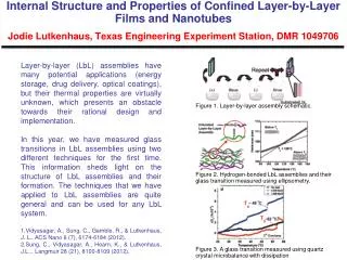
Laboratory of Computational Soft Materials. Numerical Modeling of Polyelectrolyte Adsorption and Layer-by-Layer Assembly. Qiang (David) Wang. Department of Chemical & Biological Engineering and School of Biomedical Engineering Colorado State University q.wang@colostate.edu.

E N D
Laboratory of Computational Soft Materials Numerical Modeling of Polyelectrolyte Adsorption and Layer-by-Layer Assembly Qiang (David) Wang Department of Chemical & Biological Engineering and School of Biomedical Engineering Colorado State University q.wang@colostate.edu
PE Layer-by-Layer (LbL) Assembly Decher, Science, 277, 1232 (1997) Polyelectrolytes (PE) PE are charged polymers PE are important materials • Can be soluble in water • Can be adsorbed onto charged surfaces PE are difficult to study • Both long-range (Coulomb) and short-range (excluded volume) interactions present in the system
Peyratout and Dahne, Angew. Chem. Int. Ed., 43, 3762 (2004) Why Layer-by-Layer (LbL) Assembly ? • Simple, fast, cheap • Self-healing • Versatile • Synthetic PE: conducting & light-emitting polymers, reactive polymers, polymeric complexes, polymeric dyes, … • Natural PE: DNA, RNA, proteins, viruses, … • Charged nano-particles and platelets, … • Potential Applications surface modification, enzyme immobilization, gene transfection, separation membranes, conducting or light-emitting devices, batteries, optical data storage, controlled particle and catalyst preparation, …
“Fuzzy Nanoassemblies: Toward Layered Polymeric Multicomposites” Decher, Science, 277, 1232 (1997) Black curve: Concentration profile of each layer. Blue (Red) dots: Total concentration profile of anionic (cationic) groups from all layers. Green dots: Concentration profile of a labeling group applied to every fourth layer.
A fA,b cs,b yb=0 0 x l + + + + + + Model System for PE Adsorption Parameters in the model: sSF substrate charge density; d-1 for short-range interactions between substrate and PE, >0 for repulsive and <0 for attractive substrates; p degree of ionization of PE, smeared (or annealed); c Flory-Huggins parameter between PE and solvent; fA,b bulk polymer concentration; cs,b bulk salt concentration; l system size; e (uniform) dielectric constant. solvent molecule (S) cation (+) anion (-) • Monovalent, 1D system; • Ions from salt = counterions from PE and substrate; • Ions have no volume and short-rang interactions; • Polymer segments have the same density r0 as solvent molecules; • All polymer segments have the same statistical segment length a.
Self-Consistent Field Theory (SCFT) & Ground-State Dominance Approximation (GSDA) N0: (arbitrary) chain length chosen for normalization Self-Consistent Field Theory (SCFT) Canonical ensemble H0=entropic contribution from Gaussian chains, S, +, and -; H1=short-range interaction energy described by the c parameter; H2=pure Coulomb interaction energy. Incompressibility Constraint:fA(x) +fS(x) = 1 for x ≥ 0.
Conditions for Strong Charge Inversion Attractive Attractive Repulsive Repulsive d-1=0, sSF=0.1, cs,b=0.1 sSF=0.01, cs,b=0.05, c=1 p=0.5, fA,b=1.25×10⁻⁴ p=0.5, fA,b=1.25×10⁻⁴ Poor solvent for polymers, high salt concentrations, attractive or indifferent surface for polymers, and oppositely charged surface and polyelectrolytes are all needed to obtain strong charge inversion.
cc≥1.25 GSDA vs. SCFT d-1=0, sSF=0.01, c=1, p=0.5, cs,b=0.05, fA,b=1.25×10⁻⁴ Q. Wang, MM, 38, 8911 (2005).
Layer Profiles – Symmetric, Smeared PE p1=p2=0.5, cs,b1=cs,b2=0.05 (0.667M), c1S=c2S=1 sSF=0.1 (2.61mC/m2), v1=-v2=-1, fA,b=7.5×10⁻⁴(10mM) (with a=0.5nm and r0=a-3) Q. Wang, JPC B, 110, 5825 (2006).
Layer Profiles – Symmetric, Smeared PE xw(1) p1=p2=0.5, cs,b1=cs,b2=0.05, c1S=c2S=1 Q. Wang, JPC B, 110, 5825 (2006).
Layer Profiles – Symmetric, Smeared PE p1=p2=0.5, cs,b1=cs,b2=0.05, c1S=c2S=1 Q. Wang, JPC B, 110, 5825 (2006).
Layer Profiles – Symmetric, Smeared PE p1=p2=0.5, cs,b1=cs,b2=0.05, c1S=c2S=1 Q. Wang, JPC B, 110, 5825 (2006).
Three-Zone Structure – Symmetric, Smeared PE p1=p2=0.5, cs,b1=cs,b2=0.05, c1S=c2S=1 Q. Wang, JPC B, 110, 5825 (2006).
Polymer Density in Zone II – Symmetric, Smeared PE p1=p2=0.5, cs,b1=cs,b2=0.05, c1S=c2S=cPS • Zone II is not in phase equilibrium with a bulk solution. • The total polymer density in Zone II, fPEM, does not depend on electrostatic interactions.
Charge Compensation – Smeared PE cs,b1=cs,b2=0.05, c1S=c2S=1
Charge Density Profiles –Asymmetric, Smeared PE c1S=c2S=1 p1=p2=0.5, cs,b1=cs,b2=0.05, c1S=1, c2S=0.6
Annealed vs. Smeared PE – 1st Layer p1=0.5, cs,b1=0.05, c1S=1
Charge Fractions in Multilayer – Symmetric, Annealed PE p1=p2=0.5, cs,b1=cs,b2=0.05, c1S=c2S=1 s(i): charges carried by PE adsorbed in the ith deposition. G(i): amount of PE adsorbed in the ith deposition. Each deposition changes the charges carried by the PE in a few previously deposited layers, of which the density profiles are fixed in our modeling. Thus,
Annealed vs. Smeared PE – Polymer Density in Zone II p1=p2=0.5, cs,b1=cs,b2=0.05, c1S=c2S=1
Non-Equilibrium & Solvent Effects – Symmetric, Smeared PE Multilayer does not form in q or good solvent. p1=p2=0.5, cs,b1=cs,b2=0.05, c1S=c2S=0.5, f1,b=f2,b=7.5×10⁻⁴ Q. Wang, Soft Matter, 5, 413 (2009).
Summary • We have used a self-consistent field theory to model the layer-by-layer assembly process of flexible polyelectrolytes (PE) on flat surfaces as a series of kinetically trapped states. • Our modeling, particularly for asymmetric PE having different charge fractions, bulk salt concentrations, or solvent qualities, reveals the internal structure and charge compensation of PE multilayers. We have also compared multilayers formed by strongly and weakly dissociating PE. • Our results qualitatively agree with most experimental findings. • Q. Wang, MM, 38, 8911 (2005). • Q. Wang, JPC B, 110, 5825 (2006). • Q. Wang, Soft Matter, 5, 413 (2009). q.wang@colostate.edu