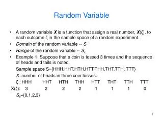
5.2 Continuous Random Variable
5.2 Continuous Random Variable. Recall Discrete Distribution. For a discrete distribution, for example Binomial distribution with n=5, and p=0.4, the probability distribution is x 0 1 2 3 4 5

5.2 Continuous Random Variable
E N D
Presentation Transcript
Recall Discrete Distribution • For a discrete distribution, for example Binomial distribution with n=5, and p=0.4, the probability distribution is x 0 1 2 3 4 5 f(x) 0.07776 0.2592 0.3456 0.2304 0.0768 0.01024
P(x) x A probability histogram
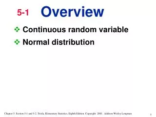
How to describe the distribution of a continuous random variable? • For continuous random variable, we also represent probabilities by areas—not by areas of rectangles, but by areas under continuous curves. • For continuous random variables, the place of histograms will be taken by continuous curves. • Imagine a histogram with narrower and narrower classes. Then we can get a curve by joining the top of the rectangles. This continuous curve is called a probability density (or probability distribution).
Continuous distributions: Density Function • For any x, P(X=x)=0. (For a continuous distribution, the area under a point is 0.) • Can’t use P(X=x) to describe the probability distribution of X • Instead, consider P(a≤X≤b)
Density Function • A probability density function for a continuous random variable X is a nonnegative function f(x) with • And such that for all a≤b, one is willing to assign P[a≤X≤b] according to
Density function • A curve f(x): f(x) ≥ 0 • The area under the curve is 1 • P(a≤X≤b) is the area between a and b
Cumulative Probability function • For X continuous with probability density f(x) • We can get the density function f(x) from F(x) by differentiation
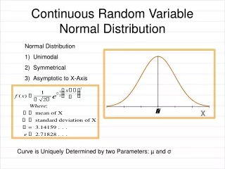
The normal distribution • A normal curve: Bell shaped • Density is given by • μand σ2are two parameters: mean and variance of a normal population (σ is the standard deviation)
Example (p323 #7) • In a grinding operation, there is an upper specification of 3.15 in. on a dimension of a certain part after grinding. Suppose that the standard deviation of this normally distributed dimension for parts of this type ground to any particular mean dimension μ is σ=.002 in. Suppose further that you desire to have no more than 3% of the parts fail to meet specifications. What is the maximum μ (minimum machining cost) that can be used if this 3% requirement is to be met?
So 3.15 is 1.88 σ above the mean. 3.15-1.88*0.002=3.146
Exponential distribution • The exponential distribution is a continuous probability distribution with • Exponential distributions are often used to describe waiting times until occurrence of events.
Mean and Variance • Mean of an exponential distribution is • Variance of the exponential distribution is
When alpha=1 P(X<2) on density curve f(x) P(X<2) on CDF F(x)
Force of Mortality Function • The force of Mortality Function is (p.760): • H(t)dt is the probability of dying in time t to t+dt if we are still living in t. • For exponential distribution • So the exponential distribution has a constant force-of-mortality.
If the lifetime of an engineering component is described using a constant force of mortality, there is no (mathematical) reason to replace such a component before it fails. • The distribution of its remaining life from any point in time is the same as the distribution of the time till failure of a new component of the same type.
Section 5.2.3 Weibull Distribution Very commonly lifetimes of motors, etc. are modeled with Weibull distributions. A Weibull distribution is a generalization of an exponential distribution and provides more flexibility in terms of distributional shape.
For component with increasing force-of-mortality (IFM) distribution, such components are retired from service once they reach a particular age, even if they have not failed.
Exercise The lifetime of a certain type of battery has an exponential distribution with average lifetime 100 hours. 5 batteries are installed at the same time and suppose that the operations of the batteries are independent. Find the probability that only 2 batteries are still working after 50 hours.