Download
1 / 37
370 likes | 619 Views
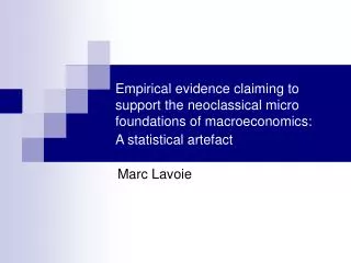
Empirical evidence claiming to support the neoclassical micro foundations of macroeconomics: A statistical artefact. Marc Lavoie. An artefact: definition. An artefact or artifact is a spurious finding caused by faulty procedures.

E N D
Empirical evidence claiming to support the neoclassical micro foundations of macroeconomics: A statistical artefact Marc Lavoie
An artefact: definition • An artefact or artifact is a spurious finding caused by faulty procedures. • In the fantasy literature, an artifact is a magical tool with great power.
INTRODUCTION -- JUSTIFICATION • Heterodox economists often claim that neoclassical production functions, substitution effects, etc., make little sense in our world of fixed coefficients and income effects. Claims to that effect also arose from the Cambridge capital controversies. • Neoclassical economists, however, have come up with a large number of empirical studies that seem to “verify” neoclassical theory, in particular when fitting Cobb-Douglas production functions (Q = eμt LαKβ). • The purpose of this lecture is to explain this apparent paradox, and show that the “good fits” of neoclassical number crunchers is no evidence at all. • Students can embrace heterodox microeconomics and its alternative assumptions without remorse: the numerous studies of empirical “evidence” supporting neoclassical production functions are worthless.
Outline • Cambridge capital (1960s) controversies anew • The equations that could verify the validity of the neoclassical theory of production and labour demand are no different from those of national accounting. • Labour theory • Lavoie 2000 • Anadyke-Danes & Godley 1989 • Production functions • McCombie 2000, McCombie and Felipe • Shaikh 1974, 2005 • Neoclassical production functions and labour demand functions are not behavioural concepts that can be empirically refuted. • Neoclassical production functions are artefacts: they claim to measure the output elasticities with respect to capital and labour, whereas in reality they are estimating the profit share and the wage share in income!
The Cambridge capital controversies • They put in jeopardy the neoclassical concepts of • Scarcity • Substitution • Marginalism • Capital as a primary factor of production • The measure of multifactor technical progress On the basis of models with fixed technical coefficients but with several techniques, or even an infinity of techniques. • These are static models, with profit maximization • These models provide cases of (See Cohen and Harcourt 2003): • Reswitching (a technique which was optimal at high interest rates, and then abandoned, becomes optimal again at low interest rates). • Capital reversal (or real Wicksell effects: a lower interest rate is associated with a technique that is less mechanized (K/L is lower), even without reswitching. • An infinitely small change in the interest rate can generate an enormous change in the K/L ratio (discontinuity, rejection of the discrete postulate).
LS w/p LD LD w/p L/K L/K Neoclassical Garegnani 1970 w/p LD L/K Garegnani 1990
The replies of neoclassical authors to the Cambridge-Sraffian arguments • Neoclassical authors minimize the capital paradoxes, making an analogy with Giffen goods in microeconomics. • They look for the conditions that would be required to keep production functions as ‘well behaved’ • They claim that general equilibrium theory is impervious to the critique. • They claim that they have the Faith, or they plead ignorance. • Empiricism (It works, therefore it exists).
Empiricism, from the very beginning • Bronfenbrenner 1971: Cobb-Douglas production functions work, not for magical reasons, but because its many applications have demonstrated that it can explain empirical facts. • Ferguson 1978: The validity of neoclassical theory is an empirical question, not a theoretical one. • Sato (1974): « The neoclassical postulate is itself in principle empirically testable in the form of a production function estimation of the CES and other varieties. This can make us go beyond purely theoretical speculations on this matter ».
Present empiricism • « The estimated elasticities that seem to confirm the central prediction of the theory of labor demand are not entirely an artefact produced by aggregating data. … The Cobb-Douglas function is not a very severe departure from reality in describing production relations» (Hamermesh 1986). • « The neoclassical production function is the cornerstone of the [neoclassical growth] theory and is used in virtually all applied aggregate analyses ».(Prescott 1998).
Two examples of how neoclassical theories of labour demand seem to be supported by empiricism (and really are not). • Layard/Nickell as revised by French authors vs Lavoie • Layard/Nickell vs Godley
The WS-PS model of Layard, Nickell and Jackman (1991) revised by Cotis, Méary and Sobczak (1998, CMS). • These studies tend to show that unemploymen rates in Europe are rising because real wages are too high relative to productivity growth. The CMS French test was: • WS : w – p = a1U + a4wedge + γt • PS : w – p = b1U + b2(q–n) + b5t • Profit-maximizing first-order conditions of a neoclassical production function, well-behaved, with diminishing returns, etc., show that the following conditions must hold in the PS equation: b1= b2 = 1 • w, p, q, n, logarithmic values • q = output; n = active population ; U = unemployment rate
But the PS equation can be also precisely derived from the national accounting identities • PQ = WL + RPK • Take the logarithmic derivative • X’ = (dX/dt)\X growth rate • P’ + Q’ = α (W’ + L’) +(1-α)(R’ + P’ + K’) • W’ – P’ = (Q’ – L’) +{(1-α)/α}(Y’ – K’ – R’) • Layard makes use of two approximations, which are : • U = (N – L)/L = x • and x = log(1+x) , when x tends towards zero • 1+x = 1+(N – L)/L = N/L • Hence U = log (N/L) = log N – log L • dU/dt = N’ – L’ or else L’ = N’ – dU/dt
PS : w – p = U + (q–n) + b5t • Hence, starting from the national accounts: • W’ – P’ = (Q’ – L’) +{(1 –α)/α}(Q’ – K’ – R’) • But since: L’ = N’ – dU/dt • W’ – P’ = dU/dt + (Q’ – N’) +{(1 –α)/α}(Q’ – K’ – R’) • Integrating, and omitting the constant, the national account equations become: • w – p = U + (q–n) + {(1 –α)/α}h.t • With: h = Q’ – K’ – R’ • This is also the PS relation, but this time extracted from the national accounts! Thus it comes as no surprise that the authors conclude that their model is « not rejected by the data ». And it not surprising that the regressions of Layard et alii allow them to verify that indeed, b1= b2 = 1.
Consequences • The empirical results drawn from the WS-PS model do not (necessarily) depend on behavioural relations based on profit maximizing with well-behaved production functions, with neutral technical progress and diminishing returns. • Quite the opposite: the correlations and signs that have been obtained rest most likely on the national income identities, and as such, they have no causal or explanatory power. • The usual estimates of the neoclassical labour demand functions are only artefacts. They are meaningless.
Further consequences • In other words, economists that use PS-WS models are only providing estimates of what the determinants of the equlibrium rate of unemployment would be (a kind of NAIRU)if the neoclassical theory of labour demand, based on aggregate production functions and decreasing returns, were valid. • These estimates cannot provide any support for neoclassical theories of equilibrium unemployment. Thus, paraphrasing Nicholas Kaldor (1972: 1239), we see that the estimates based on PS equations or similar equations can only help to « illustrate » or « decorate » neoclassical theory and its assumptions of profit-maximization, decreasing returns, and equilibrium unemployment. In no way can these estimates confirm or corroborate neoclassical theory.
A «reductio ad absurdum» proof: Godley and Anadyke-Danes (1989) • These two authors intend to demonstrate that even when, by construction, the described economy has no relationship whatsoever between employment and real wages, standard econometric analysis will seem to verify a negative relationship between employment and real wages.
Godley starts out with a markup theory based on historical costs. • PQ = (1+θ)WL • P = (1+θ)WL/Q • In logs, we have: • p = φ(w – q + l) + (1-φ)(w-1 –q-1 + l-1) • φ is the proportion of goods sold in the current period. • If φ = 1, p = (w – q + l) • l = – (w – p) + q • Right away, we see that, for a given output level, we automatically get a negative relationship between employment and real wages when prices are set through a markup. • But this negative relationship only reflects the fact, that, with a given markup, the real wage will be lower if labour productivity is lowered [(w – p) = q – l ]! • With the Layard approximation, U = n – l, we would have: • (w – p) = U + (q – n) The PS curve!
The Godley Experiment • Godley assumes, by construction, that the nominal wage, output and employment all grow independently of each other, with prices set on the basis of a lagged markup (φ =.75) • w = (1.07 + random) + w-1 • q = (1.05 + random) + q-1 • l = (1.01 + random) + l-1 • Godley gets as a regression: • l = 1.3 – 0.94 (w – p) – 0.12l-1 + .73q + .01t (7.4) (1.0) (1.0) (4.2)
l= 1.3 – 0.94 (w – p) – 0.12l-1 + .73q + .01t(7.4) (1.0) (1.0) (4.2) • Employment seems to entertain a statistically significant negative relationship with real wages, as well as a positive time trend, as Layard et alii would like it to be (note that employment does not seem to depend on output q, in contrast to what post-Keynesians would argue, and that it does not depend on past employment). • But we know that, by construction, employment is completely independent of real wages, and that current employment only depends on past employment. • Empirical studies thus manage to give support to the neoclassical theory of labour demand even in those cases where we know that, by construction, neoclassical theory is irrelevant (real wages and employment are independent of each other, while prices are set on a cost-plus basis and not on marginal principles).
But it is possible to generalize even further ….… • Neoclassical aggregate production functions are completely meaningless. • When they are correctly specified, they are necessarily confirmed, in other words they cannot be falsified. • The coefficients of the production functions of the Cobb-Douglas type, as obtained through econometric analysis, don’t measure the elasticities of factors of production: they only measure the shares of labour and profits in national income!
Several authors in the past have rejected the aggregate Cobb-Douglas functions (or other similar CES or translog functions), because they simply reproduce the identities of the national accounts: • Phelps-Brown 1957 • Simon and Levy 1963 • Shaikh 1974, 1980, 2005 • Herbert Simon 1979 • Samuelson 1979 • McCombie and Dixon 1991 • McCombie 1987, 1998, 2000, 2001 • Felipe and McCombie 2000, 2002, 2005, 2006 • (Lavoie 1987, 1992, 2000) • Fisher 1971(in his work on aggregation)
Enlightning simulations … • Fisher (1971) has shown that even if conditions of aggregation did not hold, the aggregate Cobb-Douglas function did seem to « work » properly, provided the wage share was constant enough within the set of data. Fisher concludes that one must reverse the usual argument. • Rather than saying that the wage share in national income is constant because technology is of the Cobb-Douglas type, « it ought to be said that the apparent success of the Cobb-Douglas production function must be attributed to the fact that the wage share is roughly constant ».
But here are some even more compelling « reductio ad absurdum » arguments against the neoclassical production function … • McCombie (2001) takes two firms i each producing in line with a Cobb-Douglas function • Qit = A0LαitK1- αit • With α = 0.25 (labour elasticity of output). • Inputs and outputs are identical: there is no aggregation problem (the 1971 Fisher problem is avoided). • If L and K grow through time, with no technical progress, with some random fluctuations, the econometric regression will yield an α coefficient close to 0.25 as expected. • In this case, the estimate is based on physical data, and there is no problem.
However …. • Start again with the same two firms, without technical progress, and try to estimate an aggregate production function using deflated monetary values, as must be done in macroeconomics and often in microeconomics. To do so, assume, by construction, that firms impose a markup equal to 1.33 (θ = 0.33) with P = (1+θ)WL/Q, which implies that the wage share is 75%. In this case the regression will yield an estimate of the α coefficient that turns out to be 0.75. • Thus, we started with production functions and physical data according to which the labour elasticity of production is 0.25. Yet, the estimated aggregate production function (in deflated monetary terms) tells us that this elasticity is 0.75. • In other words, estimates of aggregate production functions (both at the industry of macro levels) measure wage shares and profit shares, not the elasticities of factors of production. • These aggregate production functions are useless to provide any information about the kind of technology in use or about elasticities.
Why is this so? • Because, production functions, when they are correctly estimated, only reproduce the relationships of the national accounts. • If the wage share is approximately constant, and if technical progress is adequately estimated, one will always discover that a Cobb-Douglas production function provides a good fit. • If the wage share is not constant, then CES or translog functions will yield better fits. But these production functions are subject to the very same criticisms as the Cobb-Douglas function (Dixon and McCombie 1991). • If technical progress is misrepresented (for instance through a linear function in time, rather than by a non-linear one, the elasticity estimates will not equal the profit and wage shares, and the elasticities may even turn out to be negative.
Cobb-Douglas vs national accounts • The Cobb-Douglas function: • With constant returns to scale: α+β=1 • With factors of production paid according to their marginal productivity (w/p = dQ/dL) • With output per head and capital per head, y = Q/L et k = K/L, and calling β (beta) the capital elasticity of output, the Cobb-Douglas function yields: • log y = μt + β log k • Or in growth terms, taking the log difference, Δlog: y’ = μ + βk’ • The national accounts: • Taking the log derivative of the national accounts per unit of labour yields essentially the same result: • y’ = τ + πk’ withτ = α(w/p)’ + πr’ • Or else in logs: log y = τt + π log k • With π the profit share, α the wage share, and r the profit rate. • Thus, one is not surprised to find out that the best econometric estimates of aggregate production functions, as claimed by Jorgenson (1974), confirm that α+β=1.
TONTERIAS • HUMBUG • Shaikh 1974 (with capital per head on the horizontal axis, and output per head on the vertical axis) • Even a technology that yields capital-output ratios that look like the word HUMBUG can be represented by a Cobb-Douglas function, using the method put forth by Solow (1957).
Another « ad absurdo » proof • Shaikh (2005) shows that: • Variables generated by a Goodwin-cycle model, • with a Leontief input-output technology (fixed technical coefficients) • and constant markup pricing, • so that neither marginal productivity nor marginal cost pricing exist, • will still yield econometric estimates that seem to support the existence of a neoclassical production function with factors of production being paid at productivity, and with elasticities equal to the profit and wage shares, as neoclassical theory of perfect competition would have it, • provided technical progress is specified appropriately.
Cobb-Douglas cannot be falsified as long as technical progress is adequately represented • Sometimes the Cobb-Douglas function yields non-sensical results, and hence is not « verified », as pointed out by Lucas, Romer, and Shaikh, as shown in the following Table. • The trick is avoiding to impose a linear trend to technical progress. Rather one must introduce a non-linear trend (some sine function, or a Fournier series), because technical progress is highly variable. • Solow (1957) in his equation, y’ = μ + βk’, creates a technical progress variable which is exactly equal to: μ= α(w/p)’ + πr’, which he derived straightforwardly from the national accounts. In other words, he tested the national accounts identity, while claiming he had corroborated the neoclassical theory of income distribution, and got the Nobel Prize for this! • Indeed, nowadays, neoclassical authors that still « test » the Cobb-Douglas production function adjust the data by making corrections to the capital stock, deflating the capital index by taking into account the rate of capacity utilization, which is tightly linked to the rate of technical progress, thus obtaining a good « fit » with their regressions.
Table 1: Cobb-Douglas production functions fitted to actual and simulated aggregate data (OLS) With constant time trend: log y = cste + μt + βlog k Source: Anwar Shaikh, Eastern Economic Journal (2005)
Source: Shaikh 2005 Rate of technical change Goodwin data Rate of technical change US data
Table 2: Constant returns Cobb-Douglas functions with variable time trends for technical change (OLS) log y = cste + log At + β log k
Real wage W/P y True relationship (Leontief) yt= ρkt y2 y1 Pseudo neoclassical production function y0 R k ρ k0 k1 k2 Rate of profit Capital-labour ratio Source: Shaikh, 1990
A recap • The studies of Shaikh and those of McCombie and Felipe show that the econometric estimates of neoclassical production functions based on deflated monetary values, as is the case at the macro and industry levels when direct physical data is not used, yield pure artefacts (purely imaginary results). This affects: • Labour demand functions and NAIRU measures; • Measures of multifactor productivity (Solow residuals, technical progress); • Estimates of endogenous growth, theories of economic development; • Theories of income distribution; • Measures of output elasticities with respect to labour and capital; • Measures of potential output; • Theories of Real business cycles.
Instrumentalism at its worse • Virtually, there is nothing left of applied neoclassical macroeconomics that relies on production functions. • Instrumentalism is the philosophy of science that claims that assumptions need not be realistic, as long as they help making predictions. Instrumentalism is endorsed by the Chicago school, Milton Friedman (1953), and many neoclassical economists (often without realizing it). The VAR methodology used in time-series econometrics is another example of instrumentalism. • Neoclassical economists are pushing instrumentalism to the hilt: what counts is their ability to make predictions (based on estimates of elasticities), even if these predictions are meaningless (the estimates do not measure elasticities, but instead measure something else – profit shares and wage shares)!
Conclusion • Heterodox economists need not fear the mountain of empirical evidence that seems to support neoclassical microeconomics. • Most, perhaps all, of this evidence is an artefact. • Obviously, it follows that macroeconomics ought to be based on alternative (heterodox) foundations.
Main References • Anyadike-Danes m., Godley w. [1989], «Real wages and employment: A sceptical view of some recent econometric work», Manchester School, 57 (2), juin. • Cohen a. and Harcourt, g.c. {2003], «Whatever happened to the Cambridge capital controversies», Journal of Economic Perspectives, Winter. • Felipe j., McCombie j.s.l. [2005], «How sound are the foundations of the aggregate production function», Eastern Economic Journal, Summer 2005. • Felipe j., McCombie j.s.l. [2006], «The tyranny of the identity: growth accounting revisited», International Review of Applied Economics, 20 (3). • Garegnani p. [1990], «Quantity of Capital», in Eatwell, Millgate and Newman (eds), Capital Theory: The New Palgrave, Macmillan, 1990. • Lavoie m. [2000], « «Le chômage d’équilibre: réalité ou artefact statistique», Revue Économique, vol. 51, no. 6, Novembre, 2000, pp. 1477-1484. • McCombie j.s.l., [1998], «Are there laws of production? An assessment of the early criticisms of the Cobb-Douglas production function», Review of Political Economy, April 1998. • McCombie j.s.l., [2001], «What does the aggregate production show? Second thoughts on Solow’s “Second thoughts on growth theory”», Journal of Post Keynesian Economics, Summer. • McCombie J.S.L., Dixon R. [1991], «Estimating technical change in aggregate production functions: a critique», International Review of Applied Economics, 5 (1). • Shaikh a. [1974], «Laws of production and laws of algebra: the humbug production function», Review of Economics and Statistics, 56 (1), février. • Shaikh a. [1990], «Humbug production function», in Eatwell, Millgate and Newman (eds), Capital Theory: The new Palgrave, Macmillan, 1990. • Shaikh a. [2005], «Non-linear dynamics and pseudo production functions», Eastern Economic Journal, Summer 2005. • Simon h.a. [1979], «On parsimonious explanations of production relations», Scandinavian Journal of Economics, 81 (4).