Download
1 / 22
220 likes | 316 Views
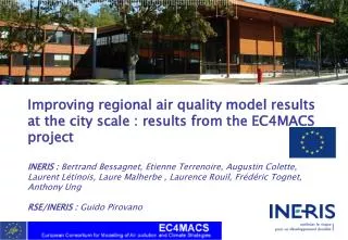
Explore how to account for the urban dimension in integrated assessment modeling by improving emissions, land use proxies, and resolution levels, using simulations and sensitivity analysis to correct model limitations.

E N D
CityDelta background • EC4MACS « urbanmodelling » component : betteraccount for the urban dimension in the integratedassessmentmodelling • What? : concentration increment (or decrement) due to the city itself • Why? : to correct coarseresolution model used in integratedassessment • How? : • Can bedefined as δ=Chigh- Clow • In the former CityDelta exercice : with a set of CTM results over 7 cities in Europe thatlead to a single formula for all Europeancities • CHIMERE highresolution (7 km) simulation over a large part of Europe [ECMWF data + WRF ; EMEP emissions]
Improvingemissions • « residentialemissions » (SNAP2) reallocatedwith population density (+ woodburningshareurban vs rural with french data) • « Crops » landuse proxy for Agricultural sector • « built-up » landuse proxy for the otheranthropogenicsectors • « roadmap » proxy for road trafficemissions (in progress) PPM2.5 emissionbefore PPM2.5 emissionafter
Inluence of vertical resolution • Three simulations performedwith CHIMERE over the Paris area • C8 : Referencerunwith 8 levels (first at 40 m) up to 500 Hpa • C20 : Simulation with 20 levels (first at 40 m) up to 500 Hpa • C9 : Simulation with 9 levels (first at 10 m) up to 500 Hpa
Inluence of vertical resolution Coll. L. Menut LMD/IPSL-CNRS
Improving horizontal resolution – why 7 km resolution? • For secondarypollutantslike O3, 12 km seems an optimal resolution (Valari and Menut , 2008) • From the POMI exercize , no gain from 6km to 3 km (even for PM) • Computing time…(increase of gridcellnumber and decrease of time step)
COARSE (50 km) The simulation domains NEST (7km) 300 x 400 grid points! • A highresolutionrunisperformed over the greydomain (7 km) (i,j) • A highresolutionrunisperformed over the greydomain • For eachsmallcell (i,j) : • the highres. conc : • the coarseres. Conc. : • the averaged concentration : • DELTA assumed to be:
Simulation results • Two simulations performed for the year 2006 : • A simulation withonlyprimaryparticulatematter and lowlevel sources (SNAP 2, 7 and partly 3) PPM run • A full chemistryrun Delta PPM2.5 species µg.m-3 2006 Month
[PPM based delta] versus [full PM based delta] µg.m-3 PPM run: Delta PPM2.5 species µg.m-3 FULLCHEM run: Delta PM2.5 species
Model underestimations • Usuallywe have an underestimate of PM • SOA formation (background issue) • Wildfires (60% of the total PM10 emissions in Europe! including a part of Russia - AQMEII project) (background issue) • Domesticwoodburning in wintertime • Road trafficresuspension • Resuspensionfromsoilerosion (background issue) • Emission vertical profiles • Meteorology (kzcalculation, wetdeposition)
PM2.5 Jan 2006 – using EMEP vertical profile for SNAP 2 emissions
PM2.5 Jan 2006 – putting all SNAP 2 in the first CHIMERE layer
Conclusion • Downscalingmethod of EMEP emissiondatasetimproved for ourhighresolution • High resolutionrunwasperformed over Europe to computecitydeltas • Improvment of CHIMERE runsat all resolutions (high and low) • Define a strategy to use « deltas » in integratedassessment model
About validation… • Pratically, itis not possible to validate a « delta » δ=Chigh- Clow; Chigh and Clow are comparable with measurements, but δ ?? • What is the order of magnitude of PM2.5 deltas? With measurements in 2009, we roughly estimate the delta =1.6 µg.m-3versus0.94 µg.m-3found in our work (for 2006). • Validation on PM2.5 for the “full chemistry run” City
Box model approximation • Reminder : a coefficient K isdefined by city as δ=K.Q • Possible implementation of a box model by city to introduce a sensitivity to meteorologicalparameter • Box model increment : • Xcity= diameter of the city (m) • Xbckg= charateristic length of the background (m) (EMEP grid compliant) • Scity= surface of the city (m²) • Sbckg= surface of the low resolution cell (m2) • Q= city emissions (kg/s) • h= ABL height • U= Wind speed at 10m (m/s)
CityDelta background – are observations useful to compute the citydelta? • Main goal is to correct a coarse EMEP simulation • Wecanconsider : δideal=Creal – Clowthen, δideal corrects the model behavior and the lack of sources (using optimal interpolation methods) • Then , δideal= δknownphysics andemissions + δmissingsources & processes • And , δideal=K.Q + δmissingsources & processes • We must correct onlywhatwe know, implementing observations in the methodologyintroduces a biasdifficult to handle in GAINS calculations What to do withthisterm? Nothing! Computed in thiswork
Background O3 (AVERAGE) ppb Background O3 (lowresol)
AQMEII project Domain-wide yearly emissions [tons/y]