Download
1 / 33
330 likes | 528 Views
Dynamic Presentation of Key Concepts Module 5 – Part 2 Op Amp Circuits with Feedback. Filename: DPKC_Mod05_Part02.ppt. Overview of this Part Op Amp Circuits with Feedback. In this part of Module 5, we will cover the following topics: Identifying Negative Feedback The Inverting Configuration

E N D
Dynamic Presentation of Key Concepts Module 5 – Part 2Op Amp Circuits with Feedback Filename: DPKC_Mod05_Part02.ppt
Overview of this PartOp Amp Circuits with Feedback In this part of Module 5, we will cover the following topics: • Identifying Negative Feedback • The Inverting Configuration • Comparison of Virtual Short Approach with Equivalent Circuit Approach
Textbook Coverage This material is introduced in different ways in different textbooks. Approximately this same material is covered in your textbook in the following sections: • Circuits by Carlson: Section 3.3 • Electric Circuits 6th Ed. by Nilsson and Riedel: Section 5.3 • Basic Engineering Circuit Analysis 6th Ed. by Irwin and Wu: Section 3.3 • Fundamentals of Electric Circuits by Alexander and Sadiku: Section 5.4 • Introduction to Electric Circuits 2nd Ed. by Dorf: Section 6.6
Solving Op Amp Circuits We have seen that we can solve op amp circuits by using two assumptions: The Two Assumptions 1) i- = i+ = 0. 2) If there is negative feedback, then v- = v+. If not, the output saturates. The key to using these assumptions is being able to determine whether the op amp has negative feedback. Remember that we have negative feedback when a portion of the output is returned to the input, and subtracted from it.
Negative Feedback Identification For ideal op amps, we can assume that the op amp has negative feedback if there is a signal path from the output to the inverting input of the op amp. We have seen that we can solve op amp circuits by using two assumptions: The Two Assumptions 1) i- = i+ = 0. 2) If there is negative feedback, then v- = v+. If not, the output saturates.
Negative Feedback Identification For ideal op amps, we can assume that the op amp has negative feedback if there is a signal path from the output to the inverting input of the op amp. Most of the time, this feedback path is provided by using a resistor between the output and the inverting input. The Two Assumptions 1) i- = i+ = 0. 2) If there is negative feedback, then v- = v+. If not, the output saturates.
Negative Feedback Identification For ideal op amps, we can assume that the op amp has negative feedback if there is a signal path from the output to the inverting input of the op amp. In general the rule is this: If, when the output voltage increases, the voltage at the inverting input also increases immediately, then we have negative feedback. The Two Assumptions 1) i- = i+ = 0. 2) If there is negative feedback, then v- = v+. If not, the output saturates.
Negative Feedback Identification For ideal op amps, we can assume that the op amp has negative feedback if there is a signal path from the output to the inverting input of the op amp. In general the rule is this: If, when the output voltage increases, the voltage at the inverting input also increases immediately, then we have negative feedback. These are two different ways of saying the same thing. However, for most students this becomes clearer once we see some examples. We will look at one example in detail in this part, and then more examples in Part 3. Go back to Overview slide.
Inverting Configuration of the Op Amp One of the simplest op amp amplifiers is called the inverting configuration of the op amp.
Inverting Configuration of the Op Amp The inverting configuration is distinguished by the feedback resistor, Rf, between the output and the inverting input, and the input resistor, Ri, between the input voltageand the inverting input. The noninverting input is grounded.
Inverting Configuration of the Op Amp Note that the feedback resistor, Rf, between the output and the inverting input, means that we have negative feedback.
Inverting Configuration of the Op Amp Note that the feedback resistor, Rf, between the output and the inverting input, means that we have negative feedback. Thus, we will have a virtual short at the input of the op amp, and we can apply our virtual-short rule, and get
Gain for the Inverting Configuration Let’s find the voltage gain, which is the ratio of the output voltage vo to the input voltage vi. To get this, let’s define two currents, ii and if.
Gain for the Inverting Configuration Next, since we know that the voltage v- is zero, we can write that the current ii is
Gain for the Inverting Configuration Following a similar approach, since we know that the voltage v- is zero, we can write that the current if is
Gain for the Inverting Configuration Next, by applying KCL at the inverting input terminal, we can write
Gain for the Inverting Configuration Finally, we solve for vo/vi, by dividing both sides by vi, and then by multiplying both sides by -Rf, and we get
Gain for the Inverting Configuration This is the result that we were looking for. As implied by our analysis of negative feedback, the gain is not a function of the op amp gain at all. The gain is the ratio of two resistor values,
Input Resistance for the Inverting Configuration Let’s find the quantity called the input resistance of this amplifier, which is defined as the Thevenin resistance seen by the source. Here, the source is the voltage source vi.
Input Resistance for the Inverting Configuration The Thevenin resistance seen by the source will be the ratio of vi/ii. We have already solved for ii, and found that
Output Resistance for the Inverting Configuration Let’s find the output resistance of this amplifier, which is defined as the Thevenin resistance seen by the load. The load is the resistor RLOAD.
Output Resistance for the Inverting Configuration The Thevenin resistance seen by the load can be found by setting all independent sources equal to zero. The voltage source thus becomes a short circuit. We then applying a test source at the output, in place of the load. We do this here, applying a current source.
Output Resistance for the Inverting Configuration Now, we are solving for vo/it, which is the output resistance, Rout. We know that v- = 0, what we call a virtual short, due to the presence of negative feedback.
Output Resistance for the Inverting Configuration Now, we are solving for vo/it, which is the output resistance, Rout. We know that v- = 0, due to the presence of negative feedback. Thus,
Output Resistance for the Inverting Configuration Now, we are solving for vo/it, which is the output resistance, Rout. We know that i- = 0, due to our first assumption. Thus,
Output Resistance for the Inverting Configuration Now, we are solving for vo/it, which is the output resistance, Rout. Next, we write KVL around the loop marked with a dashed green line. We get,
Go back to Overview slide. Output Resistance for the Inverting Configuration Now, we are solving for vo/it, which is the output resistance, Rout. Since vo = 0, we have
Testing the Virtual Short Assumption Let’s test the results we have obtained, so test the virtual short assumption. We found the gain, input resistance, and output resistance for this configuration. Let’s check our approach, by going back to the original equivalent circuit for the op amp. That is, we replace the op amp with a dependent source.
Testing the Virtual-Short Assumption We can solve this circuit for the gain, vo/vi. This requires some circuit analysis, but when we do so, we get If we take the limit as A goes to infinity, we get the same answer we had before,
Testing the Virtual-Short Assumption We can solve this circuit for the input resistance, vi/ii. This requires some analysis, but when we do so, we get If we take the limit as A goes to infinity, we get the same answer we had before,
Testing the Virtual-Short Assumption We can solve this circuit for the output resistance, vt/it, for the circuit below. This requires some analysis, but when we do so, we get In this case, we do not have to take the limit as A goes to infinity to get the same answer we had before.
Is the Virtual-Short Assumption Really Valid? • This is a good question. • You can check this by performing the solutions with actual values for real op amps. Try an open loop gain A of 106, and resistor values such as Rf = 10[kW] and Ri = 1[kW], and see how close your answers are. • You can also check this by building an op amp circuit, and measuring the actual gain, and other parameters. You mightbe surprised by how accurate the virtual-short assumption is. Go back to Overview slide.
Is the Virtual-Short Assumption Really Valid? • Strictly speaking, the answer is no. It is only an approximation. • However, it is such a good approximation, we are going to use it for the rest of this module, in all cases where negative feedback is present. Go back to Overview slide.