CSE245: Computer-Aided Circuit Simulation and Verification
370 likes | 396 Views
Explore formulation techniques, simulation approaches, and applications in computer-aided circuit analysis. Learn methods such as KCL, KVL, and conservation laws for accurate results. Dive into nonlinear systems and sensitivity analysis for comprehensive insights.

CSE245: Computer-Aided Circuit Simulation and Verification
E N D
Presentation Transcript
CSE245: Computer-Aided Circuit Simulation and Verification Lecture 1: Introduction and Formulation Winter 2013 Chung-Kuan Cheng
Administration • CK Cheng, CSE 2130, tel. 858 534-6184, ckcheng@ucsd.edu • Lectures: 5:00 ~ 6:20pm MW CSE2154 • References • 1. Electronic Circuit and System Simulation Methods, T.L. Pillage, R.A. Rohrer, C. Visweswariah, McGraw-Hill, 1998 • 2. Interconnect Analysis and Synthesis, CK Cheng, J. Lillis, S.Lin and N. Chang, John Wiley, 2000 • 3. Computer-Aided Analysis of Electronic Circuits, L.O. Chua and P.M. Lin, Prentice Hall, 1975 • 4. A Friendly Introduction to Numerical Analysis, B. Bradie, Pearson/Prentice Hall, 2005, http://www.pcs.cnu.edu/~bbradie/textbookanswers.html • 5. Numerical Recipes: The Art of Scientific Computing, Third Edition, W.H. Press, S.A. Teukolsky, W.T. Vetterling, and B.P. Flannery, Cambridge University Press, 2007. • Grading • Homework: 60% • Project Presentation: 20% • Final Report: 20%
CSE245: Course Outline • Content: • 1. Introduction • 2. Problem Formulations: circuit topology, network regularization • 3. Linear Circuits: matrix solvers, explicit and implicit integrations, matrix exponential methods, convergence • 4. Nonlinear Systems: Newton-Raphson method, Nesterov methods, homotopy methods • 5. Sensitivity Analysis: direct method, adjoint network approach • 6. Various Simulation Approaches: FDM, FEM, BEM, multipole methods, Monte Carlo, random walks • 7. Applications: power distribution networks, IO circuits, full wave analysis, Boltzmann machines
Motivation: Analysis Energy: Fission, Fusion, Fossil Energy, Efficiency Optimization Astrophysics: Dark energy, Nucleosynthesis Climate: Pollution, Weather Prediction Biology: Microbial life Socioeconomic Modeling: Global scale modeling Nonlinear Systems, ODE, PDE, Heterogeneous Systems, Multiscale Analysis.
Motivation: Analysis Exascale Calculation: 1018, Parallel Processing at 20MW • 10 Petaflops 2012 • 100 PF 2017 • 1000 PF 2022
Motivation: Analysis Modeling: Inputs, outputs, system models. Simulation: Time domain, frequency domain, wavelet simulation. Sensitivity Calculation: Optimization Uncertainty Quantification: Derivation with partial information or variations User Interface: Data mining, visualization,
Motivation: Circuit Analysis • Why • Whole Circuit Analysis, Interconnect Dominance • What • Power, Clock, Interconnect Coupling • Where • Matrix Solvers, Integration Methods • RLC Reduction, Transmission Lines, S Parameters • Parallel Processing • Thermal, Mechanical, Biological Analysis
Circuit Input and setup Simulator: Solve numerically Output Circuit Simulation • Types of analysis: • DC Analysis • DC Transfer curves • Transient Analysis • AC Analysis, Noise, Distortions, Sensitivity
Program Structure (a closer look) Input and setup Models • Numerical Techniques: • Formulation of circuit equations • Solution of ordinary differential equations • Solution of nonlinear equations • Solution of linear equations Output
Lecture 1: Formulation • Derive from KCL/KVL • Sparse Tableau Analysis (IBM) • Nodal Analysis, Modified Nodal Analysis (SPICE) *some slides borrowed from Berkeley EE219 Course
Conservation Laws • Determined by the topology of the circuit • Kirchhoff’s Current Law (KCL): The algebraic sum of all the currents flowing out of (or into) any circuit node is zero. • No Current Source Cut • Kirchhoff’s Voltage Law (KVL): Every circuit node has a unique voltage with respect to the reference node. The voltage across a branch vb is equal to the difference between the positive and negative referenced voltages of the nodes on which it is incident • No voltage source loop
Branch Constitutive Equations (BCE) Ideal elements
Formulation of Circuit Equations • Unknowns • B branch currents (i) • N node voltages (e) • B branch voltages (v) • Equations • N+B Conservation Laws • B Constitutive Equations • 2B+N equations, 2B+N unknowns => unique solution
R3 1 2 Is5 R1 R4 G2v3 0 Equation Formulation - KCL Law: State Equation: A i = 0 Node 1: Node 2: N equations Branches Kirchhoff’s Current Law (KCL)
Equation Formulation - KVL R3 1 2 Is5 R1 R4 G2v3 0 Law: State Equation: v - AT e = 0 vi = voltage across branch i ei = voltage at node i B equations Kirchhoff’s Voltage Law (KVL)
R3 1 2 Is5 R1 R4 G2v3 0 Equation Formulation - BCE Law: State Equation: Kvv + Kii = is B equations
1 2 3 j B 1 2 i N { +1 if node i is + terminal of branch j -1 if node i is - terminal of branch j 0 if node i is not connected to branch j Aij = Equation FormulationNode-Branch Incidence Matrix A branches n o d e s (+1, -1, 0)
Equation Assembly (Stamping Procedures) • Different ways of combining Conservation Laws and Branch Constitutive Equations • Sparse Table Analysis (STA) • Nodal Analysis (NA) • Modified Nodal Analysis (MNA)
Sparse Tableau Analysis (STA) • Write KCL: Ai=0 (N eqns) • Write KVL: v - ATe=0 (B eqns) • Write BCE: Kii + Kvv=S (B eqns) N+2B eqns N+2B unknowns N = # nodes B = # branches Sparse Tableau
Sparse Tableau Analysis (STA) Advantages • It can be applied to any circuit • Eqns can be assembled directly from input data • Coefficient Matrix is very sparse Disadvantages • Sophisticated programming techniques and data structures are required for time and memory efficiency
Nodal Analysis (NA) 1. Write KCL Ai=0 (N equations, B unknowns) 2. Use BCE to relate branch currents to branch voltages i=f(v) (B equations B unknowns) • Use KVL to relate branch voltages to node voltages v=h(e) (B equations N unknowns) N eqns N unknowns N = # nodes Yne=ins Nodal Matrix
1 2 Is5 R1 R4 G2v3 0 Nodal Analysis - Example R3 • KCL: Ai=0 • BCE: Kvv + i = is i = is - Kvv A Kvv = A is • KVL: v = ATe A KvATe = A is Yne = ins Yn = AKvAT Ins = Ais
Nodal Analysis • Example shows how NA may be derived from STA • Better Method: Yn may be obtained by direct inspection (stamping procedure) • Each element has an associated stamp • Yn is the composition of all the elements’ stamps
N+ i Rk N+ N- N+ N- N- Nodal Analysis – Resistor “Stamp” Spice input format: Rk N+ N- Rkvalue What if a resistor is connected to ground? …. Only contributes to the diagonal KCL at node N+ KCL at node N-
N+ NC+ + vc - NC+ NC- N+ N- Gkvc N- NC- Nodal Analysis – VCCS “Stamp” Spice input format: Gk N+ N- NC+ NC- Gkvalue KCL at node N+ KCL at node N-
N+ N- Nodal Analysis – Current source “Stamp” Spice input format: Ik N+ N- Ikvalue N+ N- N+ N- Ik
Nodal Analysis (NA) Advantages • Yn is often diagonally dominant and symmetric • Eqns can be assembled directly from input data • Yn has non-zero diagonal entries • Yn is sparse (not as sparse as STA) and smaller than STA: NxN compared to (N+2B)x(N+2B) Limitations • Conserved quantity must be a function of node variable • Cannot handle floating voltage sources, VCVS, CCCS, CCVS
Modified Nodal Analysis (MNA) How do we deal with independent voltage sources? • ikl cannot be explicitly expressed in terms of node voltages it has to be added as unknown (new column) • ek and el are not independent variables anymore a constraint has to be added (new row) Ekl k l + - l k ikl
N+ N- ik RHS Ek + - N+ N- Branch k N- ik MNA – Voltage Source “Stamp” Spice input format: Vk N+ N- Ekvalue N+
Modified Nodal Analysis (MNA) How do we deal with independent voltage sources? Augmented nodal matrix In general: Some branch currents
MNA – General rules • A branch current is always introduced as an additional variable for a voltage source or an inductor • For current sources, resistors, conductors and capacitors, the branch current is introduced only if: • Any circuit element depends on that branch current • That branch current is requested as output
+ v3 - ES6 R3 - + 3 1 2 R8 Is5 R1 R4 G2v3 - + 0 4 E7v3 MNA – An example Step 1: Write KCL (1) (2) (3) (4)
MNA – An example Step 2: Use branch equations to eliminate as many branch currents as possible (1) (2) (3) (4) Step 3: Write down unused branch equations (b6) (b7)
MNA – An example Step 4: Use KVL to eliminate branch voltages from previous equations (1) (2) (3) (4) (b6) (b7)
Modified Nodal Analysis (MNA) Advantages • MNA can be applied to any circuit • Eqns can be assembled directly from input data • MNA matrix is close to Yn Limitations • Sometimes we have zeros on the main diagonal