
Chapter 6
Time Delays. Time delays occur due to:. Fluid flow in a pipe Transport of solid material (e.g., conveyor belt) Chemical analysis Sampling line delay Time required to do the analysis (e.g., on-line gas chromatograph). Chapter 6. Mathematical description:

Chapter 6
E N D
Presentation Transcript
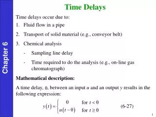
Time Delays Time delays occur due to: • Fluid flow in a pipe • Transport of solid material (e.g., conveyor belt) • Chemical analysis • Sampling line delay • Time required to do the analysis (e.g., on-line gas chromatograph) Chapter 6 Mathematical description: A time delay, , between an input u and an output y results in the following expression:
Example: Turbulent flow in a pipe Let, fluid property (e.g., temperature or composition) at point 1 fluid property at point 2 Chapter 6 Fluid In Fluid Out Point 1 Point 2 Figure 6.5 Assume that the velocity profile is “flat”, that is, the velocity is uniform over the cross-sectional area. This situation is analyzed in Example 6.5 and Fig. 6.6.
Example 6.5 For the pipe section illustrated in Fig. 6.5, find the transfer functions: (a) relating the mass flow rate of liquid at 2, w2, to the mass flow rate of liquid at 1, wt, (b) relating the concentration of a chemical species at 2 to the concentration at 1. Assume that the liquid is incompressible. Chapter 6 Solution (a) First we make an overall material balance on the pipe segment in question. Since there can be no accumulation (incompressible fluid), material in = material out
Putting (6-30) in deviation form and taking Laplace transforms yields the transfer function, (b) Observing a very small cell of material passing point 1 at time t, we note that in contains Vc1(t) units of the chemical species of interest where V is the total volume of material in the cell. If, at time t + , the cell passes point 2, it contains units of the species. If the material moves in plug flow, not mixing at all with adjacent material, then the amount of species in the cell is constant: Chapter 6 or
An equivalent way of writing (6-31) is if the flow rate is constant. Putting (6-32) in deviation form and taking Laplace transforms yields Chapter 6 Time Delays (continued) Transfer Function Representation: Note that has units of time (e.g., minutes, hours)
Two widely used approximations are: • Taylor Series Expansion: The approximation is obtained by truncating after only a few terms. Polynomial Approximations to For purposes of analysis using analytical solutions to transfer functions, polynomial approximations for are commonly used. Example: simulation software such as MATLAB and MatrixX. Chapter 6
Padé Approximations: Many are available. For example, the 1/1 approximation is, Chapter 6 Implications for Control: Time delays are very bad for control because they involve a delay of information.
Approximation of Higher-Order Transfer Functions In this section, we present a general approach for approximating high-order transfer function models with lower-order models that have similar dynamic and steady-state characteristics. In Eq. 6-4 we showed that the transfer function for a time delay can be expressed as a Taylor series expansion. For small values of s, Chapter 6
An alternative first-order approximation consists of the transfer function, Chapter 6 • where the time constant has a value of • Equations 6-57 and 6-58 were derived to approximate time-delay terms. • However, these expressions can also be used to approximate the pole or zero term on the right-hand side of the equation by the time-delay term on the left side.
Skogestad’s “half rule” • Skogestad (2002) has proposed a related approximation method for higher-order models that contain multiple time constants. • He approximates the largest neglected time constant in the following manner. • One half of its value is added to the existing time delay (if any) and the other half is added to the smallest retained time constant. • Time constants that are smaller than the “largest neglected time constant” are approximated as time delays using (6-58). Chapter 6
Example 6.4 Consider a transfer function: Derive an approximate first-order-plus-time-delay model, Chapter 6 • using two methods: • The Taylor series expansions of Eqs. 6-57 and 6-58. • Skogestad’s half rule Compare the normalized responses of G(s) and the approximate models for a unit step input.
Solution • The dominant time constant (5) is retained. Applying • the approximations in (6-57) and (6-58) gives: and Chapter 6 Substitution into (6-59) gives the Taylor series approximation,
(b) To use Skogestad’s method, we note that the largest neglected time constant in (6-59) has a value of three. • According to his “half rule”, half of this value is added to the next largest time constant to generate a new time constant • The other half provides a new time delay of 0.5(3) = 1.5. • The approximation of the RHP zero in (6-61) provides an additional time delay of 0.1. • Approximating the smallest time constant of 0.5 in (6-59) by (6-58) produces an additional time delay of 0.5. • Thus the total time delay in (6-60) is, Chapter 6
and G(s) can be approximated as: The normalized step responses for G(s) and the two approximate models are shown in Fig. 6.10. Skogestad’s method provides better agreement with the actual response. Chapter 6 Figure 6.10 Comparison of the actual and approximate models for Example 6.4.
Example 6.5 Consider the following transfer function: • Use Skogestad’s method to derive two approximate models: • A first-order-plus-time-delay model in the form of (6-60) • A second-order-plus-time-delay model in the form: Chapter 6 Compare the normalized output responses for G(s) and the approximate models to a unit step input.
Solution (a) For the first-order-plus-time-delay model, the dominant time constant (12) is retained. • One-half of the largest neglected time constant (3) is allocated to the retained time constant and one-half to the approximate time delay. • Also, the small time constants (0.2 and 0.05) and the zero (1) are added to the original time delay. • Thus the model parameters in (6-60) are: Chapter 6
(b) An analogous derivation for the second-order-plus-time-delay model gives: Chapter 6 In this case, the half rule is applied to the third largest time constant (0.2). The normalized step responses of the original and approximate transfer functions are shown in Fig. 6.11.


