Chapter 9 Computation of the Discrete Fourier Transform

1. Chapter 9 Computation of the Discrete Fourier Transform Biomedical Signal processing Zhongguo Liu Biomedical Engineering School of Control Science and Engineering, Shandong University 1 Zhongguo Liu_Biomedical Engineering_Shandong Univ.

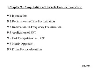
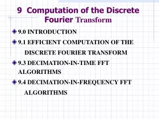
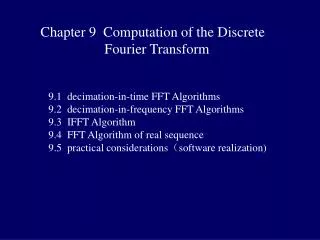
2. Chapter 9 Computation of the Discrete Fourier Transform 9.0 Introduction 9.1 Efficient Computation of Discrete Fourier Transform 9.2 The Goertzel Algorithm 9.3 decimation-in-time FFT Algorithms 9.4 decimation-in-frequency FFT Algorithms 9.5 practical considerations（software realization)

3. 1. Compute the N-point DFT and of the two sequence and • 2. Compute for • 3. Compute as the inverse DFT of 9.0 Introduction • Implement a convolution of two sequences by the following procedure: • Why not convolve the two sequences directly? • There are efficient algorithms called Fast Fourier Transform (FFT) that can be orders of magnitude more efficient than others.

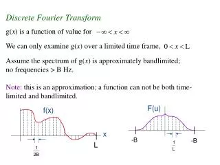
4. 9.1 Efficient Computation of Discrete Fourier Transform The DFT pair was given as • DFTcomputational complexity: • Each DFT coefficient requires • N complex multiplications; • N-1complex additions • All N DFT coefficients require • N2 complex multiplications; • N(N-1) complex additions 4

5. 9.1 Efficient Computation of Discrete Fourier Transform • Complexity in terms of real operations • 4N2 real multiplications • 2N(N-1) real additions (approximate 2N2) 5

6. 9.1 Efficient Computation of Discrete Fourier Transform Most fast methods are based on Periodicity properties Periodicity in n and k; Conjugate symmetry 6

7. 9.2 The Goertzel Algorithm Makes use of the periodicity Multiply DFT equation with this factor • Define • using x[n]=0 for n<0 and n>N-1, • X[k] can be viewed as output of a filter to input x[n] • Impulse response of filter: • X[k] is the output of the filter at time n=N 7

8. 9.2 The Goertzel Algorithm Goertzel Filter: • But it avoids computation and storage of • Computational complexity • 4N real multiplications; 4N real additions • Slightly less efficient than the direct method

9. Second Order Goertzel Filter Goertzel Filter • Multiply both numerator and denominator 9

10. Second Order Goertzel Filter Complexity for one DFT coefficient (x[n] is complex sequence). Poles: 2N real multiplications and 4N real additions Zeros: Need to be implement only once: 4 real multiplications and 4 real additions Complexity for all DFT coefficients Each pole is used for two DFT coefficients Approximately N2real multiplications and 2N2 real additions 10

11. Second Order Goertzel Filter If do not need to evaluate all N DFT coefficients Goertzel Algorithm is more efficient than FFT if less than M DFT coefficients are needed,M< log2N 11

12. 9.3 decimation-in-time FFT Algorithms Makes use of both periodicity and symmetry Consider special case of N an integer power of 2 Separate x[n] into two sequence of length N/2 Even indexed samples in the first sequence Odd indexed samples in the other sequence 12

13. 9.3 decimation-in-time FFT Algorithms • Substitute variables n=2r for n even and n=2r+1 for odd • G[k] and H[k] are the N/2-point DFT’s of each subsequence 13

14. 9.3 decimation-in-time FFT Algorithms • G[k] and H[k] are the N/2-point DFT’s of each subsequence 14

15. 8-point DFT using decimation-in-time Figure 9.3

16. computational complexity Two N/2-point DFTs 2(N/2)2 complex multiplications 2(N/2)2 complex additions Combining the DFT outputs N complex multiplications N complex additions Total complexity N2/2+N complex multiplications N2/2+N complex additions More efficient than direct DFT 16

17. 9.3 decimation-in-time FFT Algorithms Repeat same process , Divide N/2-point DFTs into TwoN/4-point DFTs Combine outputs N=8 17

18. 9.3 decimation-in-time FFT Algorithms After two steps of decimation in time • Repeat until we’re left with two-point DFT’s 18

19. 9.3 decimation-in-time FFT Algorithms flow graph for 8-point decimation in time N=2m m=log2N • Complexity: • Nlog2N complex multiplications and additions 19

20. Butterfly Computation Flow graph of basic butterfly computation • We can implement each butterfly with one multiplication • Final complexity for decimation-in-time FFT (N/2)log2N complex multiplications and Nlog2N additions 20

21. 9.3 decimation-in-time FFT Algorithms Final flow graph for 8-point decimation in time N=2m m=log2N Nlog2N complex multiplications and additions • Complexity: (Nlog2N)/2 complex multiplications and Nlog2N additions 21

22. 9.3.1 In-Place Computation同址运算 Decimation-in-time flow graphs require twosets of registers Input and output for each stage one set of registers 22

23. 9.3.1 In-Place Computation同址运算 Note the arrangement of the input indices Bit reversed indexing（码位倒置） 23

24. normal order binary coding for position： 000 001 010 011 100 101 110 111 Figure 9.13

25. cause of bit-reversed order binary coding for position： 000 001 010 011 100 101 110 111 Figure 9.13

26. 9.3.2 Alternative forms Note the arrangement of the input indices Bit reversed indexing（码位倒置） 26

27. 9.3.2 Alternative forms Figure 9.14 input in normal order and output in bit-reversed order strongpoint：in-place computations shortcoming：non-sequential access of data

28. Figure 9.15 Input, output same normal order shortcoming：not in-place computation non-sequential access of data

29. Figure 9.16 Same structure, Inputbit-reversed order , output normal order shortcoming：not in-place computation strongpoint: sequential access of data

30. 9.4 Decimation-In-Frequency FFT Algorithm The DFT equation • Split the DFT equation into even and odd frequency indexes • Substitute variables 30

31. 9.4 Decimation-In-Frequency FFT Algorithm The DFT equation 31

32. decimation-in-frequency decomposition of anN-point DFT to N/2-point DFT 32

33. decimation-in-frequency decomposition of an8-point DFT to four 2-point DFT 33

34. 2-point DFT 34

39. Final flow graph for 8-point DFTdecimation in frequency N=8 2-point DFT 4-point DFT 39

40. 9.4.1 In-Place Computation同址运算 DIF FFT DIT FFT 40

41. 9.4.1 In-Place Computation同址运算 DIF FFT transpose DIT FFT 41

42. 9.4.2 Alternative forms transpose • decimation-in-frequecyButterfly Computation • decimation-in-timeButterfly Computation 42

43. The DIF FFT is the transpose of the DIT FFT DIF FFT transpose DIT FFT 43

44. 9.4.2 Alternative forms DIF FFT transpose DIT FFT

45. 9.4.2 Alternative forms DIF FFT transpose DIT FFT

46. Figure 9.24 erratum

47. 9.4.2 Alternative forms DIF FFT transpose DIT FFT

48. Chapter 8 HW • 9.1, 9.2, 9.3, Zhongguo Liu_Biomedical Engineering_Shandong Univ. 48 上一页 下一页 返 回