Download
1 / 55
570 likes | 674 Views
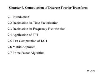
9 Computation of the Discrete Fourier Transform. 9.0 INTRODUCTION 9.1 EFFICIENT COMPUTATION OF THE DISCRETE FOURIER TRANSFORM 9.3 DECIMATION-IN-TIME FFT ALGORITHMS 9.4 DECIMATION-IN-FREQUENCY FFT ALGORITHMS. 9.0 INTRODUCTION.

E N D
9 Computation of the Discrete Fourier Transform • 9.0 INTRODUCTION • 9.1 EFFICIENT COMPUTATION OF THE DISCRETE FOURIER TRANSFORM • 9.3 DECIMATION-IN-TIME FFT ALGORITHMS • 9.4 DECIMATION-IN-FREQUENCY FFT ALGORITHMS
9.0 INTRODUCTION • The discrete Fourier transform (DFT) playing an important role in the analysis, design, and implementation of discrete-time signal-processing algorithms and systems. In this chapter , we discuss several methods for computing values of the DFT . The major focus of the chapter is a particularly efficient class of algorithms for the digital computation of the N-point DFT. Collectively , these efficient algorithms are called fast Fourier transform (FFT) algorithms, and we discuss them in Sections 9.3 and 9.4.
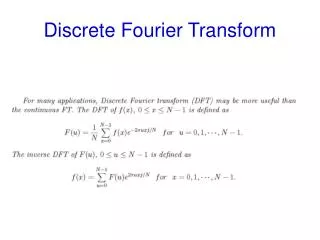
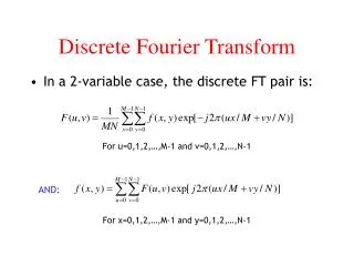
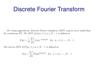
9.1 EFFICIENT COMPUTATION OF THE DISCRETE FOURIER TRANSFORM • As defined in Chapter 8 , the DFT of a finite-length sequence of length N is • where . The inverse discrete Fourier transform is given by • In Eqs.(9.1) and (9.2) , both and may be complex.
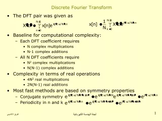
To create a frame of reference for our discussion of computation of the DFT, let us first consider direct evaluation of the DFT expression in Eq.(9.1). Since may be complex, N complex multiplications and (N-1) complex additions are required to compute each value of the DFT if we use Eq.(9.1) directly as a formula for computation. To compute all N values therefore requires a total of complex multiplications and N(N-1) complex additions.
Expressing Eq.(9.1) in terms of operations on real numbers , we • obtain • which shows that each complex multiplication requires four real multiplications and two real addition, and each complex addition requires two real additions. Therefore , for each value of k, the direct computation of requires 4N real multiplications and (4N-2) real additions. Since must be computed for N different values of k, the direct computation of the discrete Fourier transform of a sequence requires real multiplications and N(4N-2) real additions.
Most approaches to improving the efficiency of the computation • of the DFT exploit the symmetry and periodicity properties of ; specifically, • As an illustration , using the first property , i.e., the symmetry of the implicit cosine and sine functions , we can group terms in the summation in Eq.(9.3) for n and (N-n). For example
and Similar groupings can be used for the other terms inEq.(9.3) . In this way, the number of multiplications can be reduced by approximately a factor of 2.
减少了运算工作量主要利用了WNk的三个性质: (1)对称性,即 (2)周期性,即 r为任意整数。
9.3 DECIMATION-IN-TIME FFT ALGORITHMS • In computing the DFT, dramatic efficiency results from decomposing the computation into successively smaller DFT computations. In this process , we exploit both the symmetry and the periodicity of the complex exponential . Algorithms in which the decomposition is based on decomposing the sequence into successively smaller subsequences are called decimation-in-time algorithms.
The principle of the decimation-in-time algorithm is most conveniently illustrated by considering the special case of N an integer power of 2, i.e., . Since N is an even integer , we can consider computing by separating into two (N/2)-point sequences consisting of the even-numbered points in and the odd-numbered points in . With given by
and separating into its even-and odd-numbered points, we obtain or, with the substitution of variables n=2r for n even and n=2r+1 for n odd,
but , since • Consequently , Eq.(9.12) can be rewritten as • (9.14) • Each of the sums in Eq.(.14) is recognized as an (N/2)-point DFT , the first sum being the (N/2)-point DFT of the even-numbered points of the original sequence and the second being the (N/2)-point DFT of the odd-numbered points of the original sequence. • Figure 9.3 depicts this computation for N=8
Figure9.3 Flow graph of the decimation-in-time decomposition of an N-point DFT computation into two (N.2)-point DFT computations (N=8)
Equation (9.14) corresponds to breaking the original N-point • computation into two(N/2)-point DFT computations. If N/2 is even , as it is when N is equal to a power of 2, then we can consider computing each of the (N/2)-point DFTs inEq.(9.14) by breaking each of the sums in that equation into two(N/4)-point DFTs, which would then be combined to yield the (N/2)-point DFTs. Thus , G[ k] in Eq.(9.14) would be represented as • or
Similarly , H [k] would be represented as Consequently , the (N/2)-point DFT G [k] can be obtained by combining the (N/4)-point DFTs of the sequences and .
Similarly , the (N/2)-point DFT H [k] can be obtained by combining the (N/4)-point DFTs of the sequences and . • Thus , if the 4-point DFTs in Figure9.3 are computed according to Eqs.(9.16) and (9.17) , then that computation would be carried out as indicated in Figure9.4. intesing the computation of Figure9.4 into the flow graph of Figure 9.3, we obtain the complete flow graph of Figure 9.5, where we have expressed the coefficients in terms of powers rather than powers of using the fact that .
Figure 9.4. Flow graph of the decimation-in-time decomposition of an (N/2)-point DFT computation into two (N/4)-point DFT computations (N=8) • Figure 9.5 Result of substituting the structure of Figure9.4 into Figure9.3
For the 8-point DFT that we have been using as an illustration , the computation has been reduced to a computation of 2-point DFTs. For example , the 2-pint DFT of the sequence consisting of x [0] and x [4] is depicted in Figure 9.6. with the computation of Figure 9.6 inserted in the flow graph of Figure 9.5, we obtain the complete flow graph for computation of the 8-point DFT as shown in Figure9.7.
Figure 9.6 flow graph • of a 2-point DFT. Figure 9.7 Flow graph of complete decimation-in-time • decomposition of an 8-point DFT computation.
The computation in the flow graph of Figure 9.7 can be reduced further by exploiting the symmetry and periodicity of the coefficients . We first note that , in proceeding from one stage to the next in Figure9.7, the basic computation is in the form of Figure9.8, i.e., • Because of the shape of the flow graph , this elementary computation is called a butterfly . Since • the factor can be written as
With this observation , the butterfly computation of Figure 9.8 can be simplified to the form shown in Figure 9.9, which requires only one complex multiplication instead of two. Using the basic flow graph of Figure9.9 as a replacement for butterfly of the form of Figure9.8, we obtain from Figure 9.7 the flow graph of Figure 9.10.
Figure 9.9 Flow graph of simplified butterfly computation requiring only one complex Figure 9.8 Flow graph of basic Butterfly computation in Figure 9.7multiplication
Figure 9.10 Flow graph of 8-point DFT using the butterfly computation of Figure 9.9
二、运算量 任何一个N为2的整数幂(即N=2M)的DFT,都可以通过M次分解,最后成为2点的 DFT来计算。M次分解构成了从x(n)到X(k)的M级迭代计算,每级由N/2个蝶形组成。每一级运算都需要N/2次复数乘和N次复数加(每个蝶形需要两次复数加法)。所以,M级运算总共需要的复数乘次数为 复数加次数为 例如,N=210=1024时
9.3.1 In-Place Computations • The flow graph of Figure9.10 describes an algorithm for the computation of the discrete Fourier transform. The essential features of the flow graph are the branched connecting the nodes and the transmittance of each of these branches . • The particular form for the flow graph in Figure 9.10 arose out of deriving the algorithm by separating the original sequence into the even-numbered and odd-numbered points and then continuing to create smaller subsequences in the same way.
While the validity of Figure 9.10 is not tied to the order in which the input data are stored , we can order the set of complex numbers in the same order that they appear in the figure. We denote the sequence of complex numbers resulting from the mth stage of computation as , where and m=1,2,…v. furthermore , for convenience , we define the set of input samples as . We can think of as the input array and as the output array for the mth stage of the computations.
Thus, for the case of N=8, as in Figure 9.10, Figure 9.9 as indicated in Figure 9.11, with the associated equations
In order that the computation may be done in place as just discussed , the input sequence must be stored in a nonsequential order , as shown un the flow graph of Figuer 9.10. writing the indices in Eqs.(9.20) in binary form we obtain the following set of equations:
If ( n2,n1,n0) is the binary representation of the index of the sequence x [n] , then the sequence value x [n2,n1,n0] is stored in the array position X0 [n0,n1,n2] . That is , in determining the position of x [n2,n1,n0] in the input array, we must reverse the order of the bits of the index n. • Let us first consider the process depicted in Figure 9.12 for sorting a data sequence in normal order by successive examination of the bits representing the data index . If the most significant bit of the data index is zero, x [n] belongs in the half of the sorted array ; otherwise it belongs in the bottom half . Next the top half and bottom half subsequence can be sorted by examining the second most significant bit, and so on.
The tree diagrams of Figure 9.12 and 9.13 are identical , except that for normal sorting , we examine the bits representing the index from left to right , whereas for the sorting leading naturally to Figure9.7 or 9.10, we examine the bits in reverse order , right to left , resulting in bit-reversed sorting. • Figure 9.12Tree diagram depicting normal-order sorting
9.3.2 Alternative Forms • Although it is reasonable to store the results of each of the computation in the order in which the nodes appear in Figure9.10, it is certainly not necessary to do so. If we associate the nodes with indexing of an array of complex storage locations , it is clear from our previous discussion that a flow graph corresponding to an output nodes for each butterfly computation are horizontally adjacent. Otherwise two complex storage arrays will be required . Figue9.10, is , of cause , such an arrangement. Another is depicted in Figure9.14. in this case , the input sequence is in normal order and the sequence of DFT values is in bit-reversed order.
The only difference between Figures 9.10 and 9.14 is in the • ordering of the nodes. • As one example , suppose that the nodes are ordered such that the input and output both appear in normal order. A flow graph of this type is shown in Figure9.15. in this case, however , the computation cannot be carried out in place because the butterfly structure does not continue past the first stage. Thus , two complex arrays of length N would be required to perform the computation depicted in Figure9.15. • Some forms have advantages even if in-place computation is not possible. A rearrangement of the flow graph in Figure 9.10 that is particularly useful when random access memory is not available is shown in Figure9.16. this flow graph represents the decimation-in-time algorithm given by Singleton (1969). • Note first that in this flow graph the input is in bit-reversed order and the output is in normal order. The important feature of the flow graph is that the geometry is identical for each stage; only the branch transmittance change from stage to stage.
Figure 9.14 Rearrangement of figure 9.10 with input in normal order and output in bit-reversed order • .
Figure 9.15 Rearrangement of figure 9.10 with both input and output in normal order
Figure 9.16 Rearrangement of figure 9.10 having the same geometry for each stage , thereby permitting sequential data accessing and storage.
9.4 DECIMATION-IN-FREQUENCY FFT ALGORITHMS • The decimation-in-time FFT algorithms are all based on structuring the DFT computation by forming smaller and smaller subsequences of the input sequence x [n] . Alternatively , we can consider dividing the output sequence X [k] into smaller and smaller subsequences in the same manner . FFT algorithms based on this procedure are commonly called decimation-in-frequency algorithms.
To develop these FFT algorithms , let us again restrict the discussion to N a power of 2 and consider computing separately the even-numbered frequency samples and the odd-numbered frequency samples. Since the even-numbered frequency samples are • which can be expressed as
With a substitution of variables in the second summation in Eq.(9.25), we obtain Finally , because of the periodicity of
and since , Eq.(9.26)can be expressed as • Equation (9.28) is the (N/2)-point DFT of the (N/2)-point sequence obtained by adding the first half and last half of the input sequence. • We can now consider obtaining the odd-numbered frequency points , given by
As before , we can rearrange Eq.(9.29) as An alternative form for the second summation in Eq.(9.30) is
where we have used the fact that and . Substituting Eq.(9.31) into Eq.(9.30)and combing the two summations , we obtain • or, since • Equation (9.33) is the (N/2)-point DFT of the sequence obtained by subtracting the second half of the input sequence from the first half and multiplying the resulting sequence by .
The procedure suggested by eqs.(9.28) and (9.33) is illustrated for the case of an 8-pointDFT in Figure 9.17. As in the case of the procedure leading to Eqs.(9.28) and (9.33). This is accomplished by combining the first half and the last half of the input points for each of the (N/2)-point DFTs and then computing (N/4)-point DFTs. The flow graph resulting from taking this step for the 8-point example is shown in Figue 9.18.
N/2=4 点 DFT G(k) N/2=4 点 DFT H(k) -1 -1 -1 -1 • Figure 9.17 Flow graph of decimation-in-frequency decomposition of an N-point DFT computation into two (N/2)-point DFT computations (N=8).
N/4=2 DFT N/4=2 DFT -1 -1 -1 -1 N/4=2 DFT N/4=2 DFT -1 -1 -1 -1 -1 -1 Figure 9.18 Flow graph of decimation-in-frequency decomposition of an 8-point DFT computation into four 2-point DFT computations.
For the 8-point example , the computation has now been reduced • to the computation of 2-point DFTs, which are implemented by adding and subtracting the input points , as discussed previously. • Thus the 2-pint DFTs in figure 9.18 can be replaced by the computation shown in Figure 9.19, so the computation of the 8-point DFT can be accomplished by the algorithm depicted in Figure9.20. • By counting the arithmetic operations in Figure9.20 and generalizing to , we see that the computation of Figure 9.20 requires • complex multiplications and complex additions, thus the total number of computations is the same for the decimation-in-frequency and the decimation-in-time algorithms.
Figure 9.19 Flow graph of a typical 2-point DFT as required in the last stage of decimation-in-frequency decomposition.
-1 -1 -1 -1 -1 -1 -1 -1 -1 -1 -1 -1 • Figure 9.20 Flow graph of complete decimation-in-frequency decomposition of an 8-point DFT computation.
9.4.1 In-Place Computation • The flow graph in Figure 9.20 depicts one FFT algorithm based on decimation in frequency. The flow graph in Figure 9.20 begins with the input sequence in normal order and provides the output DFT in bit-reversed order, it can be interpreted as an in-place computation of the discrete Fourier transform.
9.4.2 Alternative Forms • If we denote the sequence of complex numbers resulting from the mth stage of the computation as , where and m=1,2,…v, then the basic butterfly computation show in Figure 9.21 has the form • (9.34) • By comparing Figures 9.11 and 9.21 or Wqs.(9.21) and (9.34) , we see that the butterfly computations are different for the two classes of FFT algorithms. Applying the transposition procedure to Figure 9.14 leads to Figure 9.22. • In this flow graph , the output is in normal order and the input is in bit-reversed order. Alternatively , the transpose of the flow graph of Figure 9.15 is the flow graph of Figure 9.23.