The Discrete Fourier Transform
450 likes | 772 Views
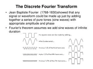
The Discrete Fourier Transform. The Fourier Transform. “The Fourier transform is a mathematical operation with many applications in physics and engineering that expresses a mathematical function of time as a function of frequency, known as its frequency spectrum.”

The Discrete Fourier Transform
E N D
Presentation Transcript
The Fourier Transform • “The Fourier transform is a mathematical operation with many applications in physics and engineering that expresses a mathematical function of time as a function of frequency, known as its frequency spectrum.” • from http://en.wikipedia.org/wiki/Fourier_transform
The Fourier Transform • “For instance, the transform of a musical chord made up of pure notes (without overtones) expressed as amplitude as a function of time, is a mathematical representation of the amplitudes and phases of the individual notes that make it up.” • from http://en.wikipedia.org/wiki/Fourier_transform
Amplitude & phase • f(x) = sin( x + ) + • is the amplitude • is the frequency • is the phase • is the DC offset
More generally • f(x) = 1 sin( 1 x + 1 ) + 2 sin( 2 x + 2 ) +
The Fourier Transform • “The function of time is often called the time domain representation, and the frequency spectrum the frequency domain representation.” • from http://en.wikipedia.org/wiki/Fourier_transform
Applications • differential equations • geology • image and signal processing • optics • quantum mechanics • spectroscopy
Complex numbers Complex numbers . . . • extend the 1D number line to the 2D plane • are numbers that can be put into the rectangular form, a+bi where i2 = -1, and a and b are real numbers.
Complex numbers Complex numbers . . . • a is the real part; b is the imaginary part • If a is 0, then a+bi is purely imaginary; if b is 0, then a+bi is a real number. • originally called “fictitious” by GirolamoCardano in the 16th century
Complex arithmetic • add/subtract • add/subtract the real and imaginary parts separately
Complex arithmetic • complex conjugate • often denoted as • negate only the imaginary part
Complex arithmetic • inverse where z is a complex number z bar is the length or magnitude of z a is the real part b is the imaginary part
Complex arithmetic • multiplication (FOIL)
Complex arithmetic • division complex conjugate of denominator
exponential vs. trigonometric (phasor form) Leonhard Euler 1707-1783
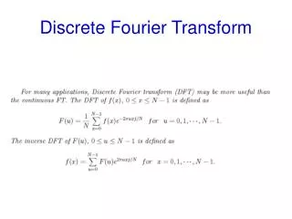
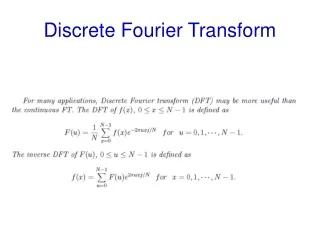
DFT • Say we have a sequence of N (possibly complex) numbers, x0 … xN-1. • The DFT produces a sequence of N (typically complex) numbers, X0 … XN-1, via the following:
DFT & IDFT • The DFT (Discrete Fourier Transform) produces a sequence of N (typically complex) numbers, X0 … XN-1, via the following: • The IDFT (Inverse DFT) is defined as follows:
Calculating the DFT So how can we actually calculate ?
Calculating the DFT • So how can we calculate ? • Let’s use this relationship: • Then • So what does this mean?
Interpretation of DFT Back to the polar form: • r/N is the amplitude and is the phase of a sinusoid with frequency k/N into which xn is decomposed
Check w/ matlab/octave % see http://www.mathworks.com/help/matlab/ref/fft.html N = 256; % # of samples n = (0:N-1); % subscripts b1 = 0.5; % freq 1 b2 = 2.5; % freq 2 xn = 0.5 * sin( b1*n ) + 0.2 * sin( b2*n ); plot( xn ); Xn = fft( xn ); plot( abs(Xn(1:N/2)) ); X0real = xn .* cos( -2*pi*n*0/N ); X0imag = xn .* sin ( -2*pi*n*0/N ); X1real = xn .* cos( -2*pi*n*1/N ); X1imag = xn .* sin ( -2*pi*n*1/N ); X2real = xn .* cos( -2*pi*n*2/N ); X2imag = xn .* sin ( -2*pi*n*2/N ); X3real = xn .* cos( -2*pi*n*3/N ); X3imag = xn .* sin ( -2*pi*n*3/N ); . . . Note: .* is element-wise (rather than matrix) multiplication in matlab.
Add random noise. % see http://www.mathworks.com/help/matlab/ref/fft.html N = 256; % # of samples n = (0:N-1); % subscripts b1 = 0.5; % freq 1 b2 = 2.5; % freq 2 r = randn( 1, N ); % noise xn = 0.5 * sin( b1*n ) + 0.2 * sin( b2*n ) + 0.5 * r; plot( xn ); Xn = fft( xn ); plot( abs(Xn(1:N/2)) ); X0real = xn .* cos( -2*pi*n*0/N ); X0imag = xn .* sin ( -2*pi*n*0/N ); X1real = xn .* cos( -2*pi*n*1/N ); X1imag = xn .* sin ( -2*pi*n*1/N ); X2real = xn .* cos( -2*pi*n*2/N ); X2imag = xn .* sin ( -2*pi*n*2/N ); X3real = xn .* cos( -2*pi*n*3/N ); X3imag = xn .* sin ( -2*pi*n*3/N ); . . .
Signal with noise. FFT of noisy signal (two major components are still apparent).
Example of differences in phase. xn = 0.5 * sin( b1*n ) + 0.2 * sin( b2*n ) xn = 0.5 * sin( b1*n – 0.5 ) + 0.2 * sin( b2*n )
Computational complexity:DFT vs. FFT • The DFT is O(N2) complex multiplications. • In 1965, Cooley (IBM) and Tukey (Princeton) described the FFT, a fast way (O(N log2 N)) to compute the FT using digital computers. • It was later discovered that Gauss described this algorithm in 1805, and others had “discovered” it as well before Cooley and Tukey. • “With N = 106, for example, it is the difference between, roughly, 30 seconds of CPU time and 2 weeks of CPU time on a microsecond cycle time computer.” – from Numerical Recipes in C
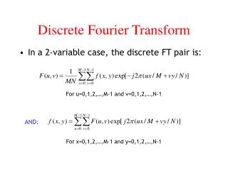
Extending the DFT to 2D(and higher) • Let f(x,y) be a 2D set of sampled points. Then the DFT of f is the following: • (Note that engineers often use i for amps (current) so they use j for -1 instead.)
Extending the DFT to 2D(and higher) • In fact, the 2D DFT is separable so it can be decomposed into a sequence of 1D DFTs. • And this can be generalized to higher and higher dimensions as well.
The classical “Gibbs phenomenon” • Visit http://en.wikipedia.org/wiki/Square_wave. • Hear it at http://www.youtube.com/watch?v=uIuJTWS2uvY.