Download
1 / 15
170 likes | 398 Views
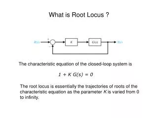
A Few Points to Make (Zeros/Poles, Root Locus, Steady-state error). Get roles of players right.

E N D
A Few Points to Make(Zeros/Poles, Root Locus, Steady-state error)
Get roles of players right I noticed the first day that some people had the roles of the different loop components wrong—the plant talking to the actuator or the controller talking directly to the plant. These roles have to be correct for the loop model to be correct.
System poles and zeros The poles of a system are the values of s that make its denominator 0. The zeros of a system are the values of s that make its numerator 0.
System poles and zeros How a system responds dynamically depends upon the location of its closed-loop poles, primarily. These can be gotten from the characteristic equation of the closed-loop system. Often, however, it is useful to deal with a system’s open-loop poles and zeros…
Poles and zeros – example Open-loop poles at s = -1/5, -1/3, -4 Open-loop zeros at s = -1/7
Poles and zeros – example Closed-loop zeros: s = -1/7, -4 Closed-loop poles depend on the value of KP. If KP = 0, s = -1/5, -1/3, -4 If KP = ∞, s= -1/7 If KP = 1, s= -3.38, -1, -0.158 (from Matlab roots() function)
CL-pole migration with changing KP As KP changes, closed-loop poles change their location. Thus by changing KP, you can change the way the closed-loop system responds.
Root locus Actually this migration of poles is covered in Chapter 7 of my book, which we are going to skip. You can see how the poles migrate quickly by using a Matlab tool called rltool(). “rl” stands for “root locus”. “locus” means “place” in Latin. So the root locus is “where the roots are”. It’s the path that they follow as you increase K.
rltool() example To use rltool(), use the open-loop transfer function. With the previous example You first create a system variable in Matlab: >> s = tf(‘s’)
rltool() example Then >> gol = (7*s+1)/((3*s+1)*(5*s+1) *(0.25*s+1)) Then >> rltool(gol) Try this and see what happens.
Root locus Thus we can use the controller to drive the roots where we want them for a particular system response. A few tips: The further to the left the closed-loop poles are, the faster the system is. If there are any roots in the right half-plane, the system is unstable and will blow up.
Root locus A system oscillates if it has complex roots. If it has no complex roots, it does not oscillate. A system is no faster than its slowest pole(s). So the right-most pole(s) generally govern the behavior of the system.
Steady-state error, ess Sometimes you tell a plant where to go and it doesn’t exactly go there. Why is this? Give cruise-control example. Table 6.1 (use GOL):