Ensemble Kalman Filter

1. Ensemble Kalman Filter Dusanka Zupanski CIRA/Colorado State University Fort Collins, Colorado Guest Lecture at AT 753: Atmospheric Water Cycle 21 April 2006, CSU/ATS Dept., Fort Collins, CO Acknowledgements: M. Zupanski, C. Kummerow, S. Denning, and M. Uliasz, CSU A. Hou and S. Zhang, NASA/GMAO Dusanka Zupanski, CIRA/CSU Zupanski@CIRA.colostate.edu

2. OUTLINE • Why Ensemble Data Assimilation? • Kalman filter and Ensemble Kalman filter • Maximum likelihood ensemble filter (MLEF) • Examples of MLEF applications • Future research directions Dusanka Zupanski, CIRA/CSU Zupanski@CIRA.colostate.edu

3. Why Ensemble Data Assimilation? Three main reasons : • Need for optimal estimate of the atmospheric state + verifiable uncertainty of this estimate; • Need for flow-dependent forecast error covariance matrix; and • The above requirements should be applicable to most complex atmospheric models (e.g., non-hydrostatic, cloud-resolving, LES). Dusanka Zupanski, CIRA/CSU Zupanski@CIRA.colostate.edu

4. Benefits of Flow-Dependent Background Errors (From Whitaker et al., THORPEX web-page) Example 1: Fronts Example 2: Hurricanes

5. Are there alternatives? Two good candidates: • 4d-var method: It employs flow-dependent forecast error covariance, but it does not propagate it in time. • Kalman Filter (KF): It does propagate flow-dependent forecast error covariance in time, but it is too expensive for applications to complex atmospheric models.  EnKF is a practical alternative to KF, applicable to most complex atmospheric models.  A bonus benefit: EnKF does not use adjoint models! Dusanka Zupanski, CIRA/CSU Zupanski@CIRA.colostate.edu

6. Maximum Likelihood Ensemble Filter Typical EnKF Forecast error Covariance Pf (ensemble subspace) Observations First guess Hessian preconditioning Non-Gaussian PDFs DATA ASSIMILATION Analysis error Covariance Pa (ensemble subspace) Optimal solution for model state x=(T,u,v,f, ) Tb,ub,vb,fb, ,, ENSEMBLE FORECASTING INFORMATION CONTENT ANALYSIS Dusanka Zupanski, CIRA/CSU Zupanski@CIRA.colostate.edu

7. Data Assimilation Equations GOAL: Combine Model and Data to obtain optimal estimate of dynamical state x Equations in model space: - Time step index - Dynamical model for model state evolution (e.g., NWP model) - Dynamical model for state dependent model error - Model state vector of dim Nstate ; - Model error vector of dim Nstate Prior (forecast) error covariance of x (assumed known): ; - Mathematical expectation Model error covariance (assumed known): Dusanka Zupanski, CIRA/CSU Zupanski@CIRA.colostate.edu

8. Data Assimilation Equations Equations in data space: - Time step index (denoting observation times) - Observations vector of dim Nobs ; - Observation operator - Observation error Observation error covariance, includes also representatives error (assumed known): Data assimilation should combine model and data in an optimal way. Optimal solution z can be defined in terms of optimal initial conditions xa(analysis), model error w, and empirical parameters ,,. Dusanka Zupanski, CIRA/CSU Zupanski@CIRA.colostate.edu

9. How can we obtain optimal solution?Two approaches are used most often: Approach 1: Optimal solution (e.g., analysis xa) = Minimum variance estimate, or conditional mean of Bayesian posterior probability density function (PDF) (e.g., Kalman filter; Extended Kalman filter; EnKF) - PDF xa is defined as mathematical expectation (i.e., mean) of the conditional posterior p(x|y), given observations y and prior p(x). Assuming liner M and H and independent Gaussin PDFs Kalman filter solution (e.g., Jazwinski 1970) For non-liner M or H the solution can be obtained employing Extended Kalman filter, or Ensemble Kalman filter. Dusanka Zupanski, CIRA/CSU Zupanski@CIRA.colostate.edu

10. Approach 2: Optimal solution (e.g., analysis xa) = Maximum likelihood estimate, or conditional mode of Bayesian posterior p(x|y)(e.g., variational methods; MLEF) xa= Maximum of posterior p(x|y), given observations and prior p(x). For independent Gaussian PDFs, this is equivalent to minimizing cost function J: Solution can be obtained (with ideal preconditioning) in one iteration for linerH and M. Iterative solution for non-linearH and M: - Preconditioning matrix = inverse Hessian of J Dusanka Zupanski, CIRA/CSU Zupanski@CIRA.colostate.edu

11. VARIATIONAL MLEF Ideal Hessian Preconditioning Milija Zupanski, CIRA/CSU ZupanskiM@CIRA.colostate.edu

12. Gaussian Non-Gaussian p(x) p(x) x x xmean xmode xmode = xmean MEAN vs. MODE Minimum variance estimate= Maximum likelihood estimate! For Gaussian PDFs and linearH and M results of all methods [KF, EnKF (with enough ensemble members), and variational] should be identical, assuming the same Pf, R,and y are used in all methods. Dusanka Zupanski, CIRA/CSU Zupanski@CIRA.colostate.edu

13. Does this really happen?!? KF, EnKF, 4d-var, all created equal?

14. TEST RESULTS EMPLOYING A LINEAR MODEL AND GAUSSIAN PDFs (M.Uliasz) (D. Zupanski)

15. Kalman filter solution Analysis step: - Optimal estimate of x (analysis) - Background (prior) estimate of x - Analysis (posterior) error covariance matrix (Nstate x Nstate) - Kalman gain matrix (Nstate x Nobs) Forecast step: ; Often neglected - Update of forecast error covariance Dusanka Zupanski, CIRA/CSU Zupanski@CIRA.colostate.edu

16. Ensemble Kalman Filter (EnKF) solution EnKF as first introduced by Evensen (1994) as a Monte Carlo filter. Equations given here following Evensen (2003) Analysis step: Analysis solution defined for each ensemble member i: Analysis ensemble perturbations: Mean analysis solution: Analysis error covariance in ensemble subspace: Sample analysis covariance

17. Ensemble Kalman Filter (EnKF) Forecast step: Ensemble forecasts employing a non-linear model M Forecast error covariance calculated using ensemble perturbations: ; Non-linear forecast perturbations Sample forecast covariance

18. There are many different versions of EnKF • Monte Carlo EnKF (Evensen 1994; 2003) • EnKF (Houtekamer et al. 1995; 2005; First operational version) • Hybrid EnKF (Hamill and Snyder 2000) • EAKF (Anderson 2001) • ETKF (Bishop et al. 2001) • EnSRF (Whitaker and Hamill 2002) • LEKF (Ott et al. 2004) Minimum variance solution Maximum likelihood solution • MLEF (Zupanski 2005; Zupanski and Zupanski 2006) Why maximum likelihood solution? It is more adequate for employing non-Gaussian PDFs (e.g., Fletcher and Zupanski 2006).

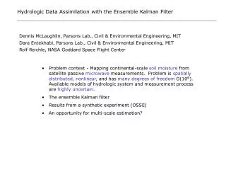
19. Current status of EnKF applications • EnKF is operational in Canada, since January 2005 (Houtekamer et al.). Results comparable to 4d-var. • EnKF is better than 3d-var (experiments with NCEP T62 GFS) - Whitaker et al., THORPEX presentation ). • Very encouraging results of EnKF in application to non-hydrostatic, cloud resolving models (Zhang et al., Xue et al.). • Very encouraging results of EnKF for ocean (Evensen et al.), climate (Anderson et al.), and soil hydrology models (Reichle et al.). Theoretical advantages of ensemble-based DA methods are getting confirmed in an increasing number of practical applications.

20. Examples of MLEF applications Dusanka Zupanski, CIRA/CSU Zupanski@CIRA.colostate.edu

21. Maximum Likelihood Ensemble Filter (Zupanski 2005; Zupanski and Zupanski 2006) - Dynamical model for standard model state x - Dynamical model for model error (bias) b - Dynamical model for empirical parameters  Define augmented state vector z , . And augmented dynamical model F  Find optimal solution (augmented analysis) zaby minimizing J (MLEF method): Dusanka Zupanski, CIRA/CSU Zupanski@CIRA.colostate.edu

22. Bias estimation: Respiration bias R, using LPDM carbon transport model (Nstate=1800, Nobs=1200, DA interv=10 days) 40 Ens Cycle 3 Cycle 1 Cycle 7 100 Ens True R Domain with larger bias (typically land) Domain with smaller bias (typically ocean) Both the magnitude and the spatial patterns of the true bias are successfully captured by the MLEF.

23. Information measures in ensemble subspace (Bishop et al. 2001; Wei et al. 2005; Zupanski et al. 2006, subm. to MWR) - information matrix in ensemble subspace of dim Nens x Nens for linear H and M - are columns of Z - control vector in ensemble space of dim Nens - model state vector of dim Nstate >>Nens Degrees of freedom (DOF) for signal (Rodgers 2000): - eigenvalues of C Shannon information content, or entropy reduction Errors are assumed Gaussian in these measures. Dusanka Zupanski, CIRA/CSU Zupanski@CIRA.colostate.edu

24. GEOS-5 Single Column Model: DOF for signal(Nstate=80; Nobs=80, seventy 6-h DA cycles, assimilation of simulated T,q observations) DOF for signal varies from one analysis cycle to another due to changes in atmospheric conditions. 3d-var approach does not capture this variability. RMS Analysis errors for T, q:------------------------------------ 10ens ~ 0.45K; 0.377g/kg 20ens ~ 0.28K; 0.265g/kg40ens ~ 0.23K; 0.226g/kg80ens ~ 0.21K; 0.204g/kg-------------------------------------No_obs ~ 0.82K; 0.656g/kg T obs (K) q obs (g kg-1) Small ensemble size (10 ens), even though not perfect, captures main data signals. Vertical levels Data assimilation cycles Dusanka Zupanski, CIRA/CSU Zupanski@CIRA.colostate.edu

25. Non-Gaussian (lognormal) MLEF framework: CSU SWM (Randall et al.) Cost function derived from posterior PDF ( x-Gaussian, y-lognormal): Lognormal additional nonlinear term Normal (Gaussian) Beneficial impact of correct PDF assumption – practical advantages Dusanka Zupanski, CIRA/CSU Zupanski@CIRA.colostate.edu Courtesy of M. Zupanski

26. Future Research Directions • Covariance inflation and localization need further investigations: Are these techniques necessary? • Model error and parameter estimation need further attention: Do we have sufficient information in the observations to estimate complex model errors? • Information content analysis might shed some light on DOF of model error and also on the necessary ensemble size. • Non-Gaussian PDFs have to be included into DA (especially for cloud variables). • Characterize error covariances for cloud variables. • Account for representativeness error. Dusanka Zupanski, CIRA/CSU Zupanski@CIRA.colostate.edu

27. References for further reading Anderson, J. L., 2001: An ensemble adjustment filter for data assimilation. Mon. Wea. Rev.,129, 2884–2903. Fletcher, S.J., and M. Zupanski, 2006: A data assimilation method for lognormally distributed observational errors. Q. J. Roy. Meteor. Soc. (in press). Evensen, G., 1994: Sequential data assimilation with a nonlinear quasi-geostrophic model using Monte Carlo methods to forecast error statistics. J. Geophys. Res., 99, (C5),. 10143-10162. Evensen, G., 2003: The ensemble Kalman filter: theoretical formulation and practical implementation. Ocean Dynamics. 53, 343-367. Hamill, T. M., and C. Snyder, 2000: A hybrid ensemble Kalman filter/3D-variational analysis scheme. Mon. Wea. Rev.,128, 2905–2919. Houtekamer, Peter L., Herschel L. Mitchell, 1998: Data Assimilation Using an Ensemble Kalman Filter Technique. Mon. Wea. Rev.,126, 796-811. Houtekamer, Peter L., Herschel L. Mitchell, Gerard Pellerin, Mark Buehner, Martin Charron, Lubos Spacek, and Bjarne Hansen, 2005: Atmospheric data assimilation with an ensemble Kalman filter: Results with real observations. Mon. Wea. Rev., 133, 604-620. Ott, E., and Coauthors, 2004: A local ensemble Kalman filter for atmospheric data assimilation. Tellus.,56A, 415–428. Tippett, M. K., J. L. Anderson, C. H. Bishop, T. M. Hamill, and J. S. Whitaker, 2003: Ensemble square root filters. Mon. Wea. Rev.,131, 1485–1490. Whitaker, J. S., and T. M. Hamill, 2002: Ensemble data assimilation without perturbed observations. Mon. Wea. Rev.,130, 1913–1924. Zupanski D. and M. Zupanski, 2006: Model error estimation employing an ensemble data assimilation approach. Mon. Wea. Rev. 134, 1337-1354. Zupanski, M., 2005: Maximum likelihood ensemble filter: Theoretical aspects. Mon. Wea. Rev., 133, 1710–1726 Dusanka Zupanski, CIRA/CSU Zupanski@CIRA.colostate.edu

28. Thank you. Dusanka Zupanski, CIRA/CSU Zupanski@CIRA.colostate.edu