Sample size calculations for cross-classified models
300 likes | 482 Views
Sample size calculations for cross-classified models. William Browne, Mousa Golalizadeh and Richard Parker University of Bristol. Contents. Sample size background Brief description of MLPowSim Fife dataset and model Balanced data

Sample size calculations for cross-classified models
E N D
Presentation Transcript
Sample size calculations for cross-classified models William Browne, Mousa Golalizadeh and Richard Parker University of Bristol
Contents • Sample size background • Brief description of MLPowSim • Fife dataset and model • Balanced data • Potential ways to factor unbalanced data into sample size calculations • Simple design effect formula for cross-classified model.
Background • Many quantitative social science research questions are of the form of a hypothesis – A has a significant effect on B. • To answer such a question data is collected that allows the researcher to (hopefully) test whether statistically A has a significant effect on B. (In fact we aim to reject the hypothesis that A doesn’t significantly affect B). • A test is performed and either the researcher is happy and A indeed has a significant effect on B or is left wondering why the data collected do not back up their hypothesis. Is the hypothesis false or was the data not sufficient? • The sufficiency of the data is the motivation for sample size calculations.
Example • Suppose I have the research question ‘Are Welshmen on average taller than 175 cms?’ • I now need to get hold of a random sample of n Welshmen and measure each of their heights. • I make some statistical assumption about the distribution of the heights of Welshmen e.g. that they come from a Normal distribution. • I might like to check this assumption by plotting a histogram of the data. • I can then form a statistical hypothesis test and test whether indeed Welshmen are taller than 175cms. • I need to decide how big to make n, my sample of Welshmen.
Hypothesis Testing • Let us assume our null hypothesis is that the average height of Welshmen (μ) is 175cm. • So we test H0:μ=175 vs HA:μ>175 (or alternatively H0:θ=0 vs HA:θ>0 where θ=μ-175) • In practice we calculate from our sample its mean ( ) and standard deviation (s2) and use these along with n to form a test statistic which we can compare with the distribution assumed under H0
Type I and Type II errors • No hypothesis test is perfect and there is always the possibility of errors • P(Type I error) = α = significance level or size • P(Type II error) = β, 1-β is the power of the test. • In general we fix α to some value e.g. 0.05, 0.01 then 1-β depends on our sample size.
Example hypothesis test • Let us assume that in reality our sample mean is 180cms and the population standard deviation (sd) is 5cms (known). • We can then form a test statistic as follows: • Note here that for small n and unknown sd we should use a student-t distribution rather than Normal. • For a 1-sided Z test we wish Z= > 1.645 and so we need our sample to be of size 3 to reject H0, using a student-t distribution increases this to 5. (Here α=0.05) • However if the sample mean had been only 176cms then we would need n > (1.645*5)2 = 68 Welshmen to reject H0
Power calculations • Our last slide in some sense is backwards as we cannot get from a given sample mean to choosing a sample size! • What we do instead is use different terminology and play God! • We will choose an ‘effect size’, γ which will represent a guess at the increase in the sample mean for Welshmen. • There then exists an (approximate) formula that links four quantities, size (α), power (1-β), effect size (γ) and sample size (n) • Note that the standard error (SE) of γ is a function of n and σ the population sd which is assumed known. • We can now evaluate one of these quantities conditional on the others e.g. what sample size is required given α,1-β and γ? Here RHS is sum of cases H0 true and H0 false.
Welsh height example Here we have looked at two examples with effect sizes 5 and 1 respectively. Assume σ takes the value 5 and so let us suppose we take a sample of size 25 Welshmen. Then Case 1: 5/(5/√25)=1.645+z1-β,z1-β=3.355 β=0.9996 Case 2: 1/(5/ √25)=1.645+z1-β,z1-β=-0.645 β=0.25946 So here a sample of 25 Welshmen from a population with mean 180cms would almost always result in rejecting H0, but if the population mean is 176cms then only 26% of such samples would be rejected. We can plot curves of how power increases with sample size as shown in the next slide.
Power curve for Welshmen example Here we see the two power curves for the two scenarios:
Extending the idea • The simple formula can be used in many situations and hypothesis tests. • To generalise the idea we assume that γ is an effect size associated with a statistic that we wish to compare with a (null) hypothesized value of 0. • The complication occurs in finding a formula for the standard error for the statistic and relating this formula to the sample size, n. • We will next consider an alternative approach before returning to look at how both approaches can be extended to cross-classified models.
The use of simulation • In reality our (hoped for) research path will be as follows: Construct research question -> Form null hypothesis that we believe false -> Collect appropriate data -> Reject hypothesis therefore proving our research question. • Assuming what we believe our research question is correct and hence the null hypothesis is false we can still be let down by not collecting enough data. • The idea behind using simulation is to simulate the data gathering process (assuming we know the right answer) many times and see how often we can reject the null hypothesis. The percentage of rejected null hypotheses (via simulation) will then estimate power.
Simulation in our example • Consider our Welsh height example case 2 where we believe Welshmen have a mean height of 176cms (and sd = 5cms) and we are testing the hypothesis H0:μ=175cms, and we consider a sample size 25. • Then we generate N samples (e.g. 5000) of size 25, • and for each sample form a lower bound for the confidence interval of the form • . This we compare with the value 175 and the proportion greater than 175 is an estimate of the power of the test. • We can repeat this exercise for different sample sizes and form a power curve.
Power curve comparison Note simulation curve is a good approximation of the theoretical curve although there are some minor (Monte Carlo) errors even with 5000 simulations per sample size.
Advantages/Disadvantages • Theoretical approach is quick when the formula can be derived. • Approximations for more complex situations exist which are equally quick. • Simulation approach generalizes to more situations but is much slower and we may need large numbers of simulations per scenario to get accurate power estimates. • Note that alternative, Standard error based method, typically needs less simulations per scenario for the same accuracy and works for normal responses.
MLPowSim software package • Software package recently completed. • A ‘rather old fashioned’ text-based interface allows user to specify sample size scenarios. • Software then generates either MLwiN macro code or an R command file to run the simulations to calculate power for scenarios. • Normal, Binomial and Poisson response offered. • Software will cope with 1-level, 2-level (balanced and unbalanced), 3-level nested (balanced and unbalanced) and cross-classified (balanced and unbalanced) with 2 higher classifications models. • Many options for unbalanced designs. • Extensive user manual (~150 pages with lots of examples) • See http://seis.bris.ac.uk/~frwjb/esrc.html for details
Cross-classified example –Fife dataset Dataset taken from the MLwiN user’s guide. Basic structure is 3,435 pupils from 19 secondary schools who also have primary school (of which there are 148) recorded. We will use this as basis for sample size calculations and use a simple variance components model Our response, Exam attainment at 16 is then modelled simply as a constant plus a secondary school effect plus a primary school effect plus a residual. Our problem is how would one perform a power calculation for this or a similar scenario?
Fife data – Balanced design? • Estimates from data: • We will begin by trying a balanced design where we have p pupils in each combination of secondary school (SS) and primary school (PS) with ns secondary and np primary schools. • Clearly balanced data inappropriate as we will not in reality get balanced data • Here we try 3 pupils in each combination of ns and np with ns = {10,20,30} and np={20,40,60,80,100}. • Note for 30 SS each PS must have at least 90 pupils which is not really feasible!
Balanced design results Results using MLPowSim and lmer in R. Note a power of > 0.8 is reached with 20 SS and 100 PS or 30 SS and 80 PS (3 pupils per pairing) = 6,000 and 7,200 pupils. Note reducing to 1 pupil per pairing has little impact on power.
Methods to include imbalance in power calculations MLPowSim offers several options: • Non-response of single observations. • Dropout of whole groups. • Sampling from a secondary school/primary school look up table. • Sampling from a pupil look up table.
Methods 1 & 2 Non response of individuals (with fixed probability) and dropout of some pairings of SS and PS are useful in other situations but not so much here. Using these options in MLPowSim shows: • 50% dropout of individuals reduces power but not greatly. • 50% dropout of pairings similarly reduces power but not greatly. This is in line with the observation that reducing the # of pupils per pairing as opposed to # of SS or PS only has a small impact on power. Basically neither of 1 and 2 removes whole SS or PS from the data which has a far greater impact on power
Method 3 – fixed sample from secondary (or primary) schools Here the idea is to imagine a design where we have balance across SS i.e. our sampling strategy is to sample n pupils from each SS. Then the PS identifier for each pupil is discovered at a later date and is not part of the sampling scheme (and is (in MLPowSim) in effect sampled from the distribution within that SS). To run this method MLPowSim requires a file giving relative numbers of pupils for each PS/SS combination. For our example we will use the actual numbers from the real data. Essentially we mimic the scenario of balance within SS which is a plausible sampling scheme. Note: We can also do the alternative of balance across PS.
Method 3 results - SS Here we see a gradual rise in power as we increase the # of pupils per SS as this in turn increases # of PS. It however takes a rather large number of pupils per SS to ensure all PS are in the simulation, and hence the number required to reach a power of 0.8
Method 3 results - PS Here we see a steep rise in power for small samples in each primary school followed by a fairly flat curve as adding more pupils doesn’t increase number of SS as all are captured with only a small number of pupils per PS.
Method 4 – fixed sample from whole population Here we take method 3 one step further and assume we take a random sample of pupils from our overall sampling frame without stratifying by either SS or PS. Here after each pupil is selected it’s SS and PS are then recorded. In our example we use the actual data as a sampling frame and so the probability of a pupil coming from each pairing is proportional to the number from that pairing in the dataset. This should result in simulated datasets that are similar in form to the true dataset.
Model 4 Results Here we see as with method 3 that power initially increases at a fast rate but after a while each dataset will contain most, if not all, of the SS and PS and then the rate slows and it takes a large number of pupils for the power to reach 0.8
Design effect formula (2 level model) • If we assume balance then with n pupils in each of N schools for a simple VC model (and only this simple model) the following formula holds: • Design effect = 1 + (n-1)ρ where ρ is the intra-class correlation. • So if we know the simple random sampling (SRS) sample size required for a given power we need to multiply this by the design effect. • For example if ρ=0.1 then for schools of size 10 pupils we would need 1+9*0.1=1.9 times as many students (in total) to get the same power. • So if for example we found that SRS requires 300 pupils then for schools of size 10 we require 1.90*300=570 pupils or 57 schools. • This can be shown to fit the simulated results.
Proposed formula for Cross classified models • We here propose an extension for cross-classified models (VC only). • Design effect: • Here we are assuming balance and all terms need defining:
DE formulae for XC models • Formulae appears to mimic behaviour noted in simulation methods, in particular in our examples, the number of pupils per school pairing has little impact on power. As the two n terms involve numbers of clusters increasing the number of SS or PS will also increase the DE and so solving is more difficult than in the hierarchical case! Of course there are multiple combinations of SS and PS that solve the problem!
Summary • We have discussed sample size calculations in general and shown results specific to cross-classified models • We welcome feedback from users of MLPOWSIM. • We offer methods (via simulation) for dealing with non-balanced data which may be more of an issue in cross-classified models. • We have tentatively proposed a simple formulae so that some of heavy computations for the simulation method can be removed in simple cases.