Sample Size calculations in multilevel modelling
Sample Size calculations in multilevel modelling. William Browne University of Nottingham (With thanks to Mousa Golalizadeh and Lynda Leese). Summary. Introduction to sample size calculations. A simulation-based approach. PINT for balanced 2 level models. Effect of balance.

Sample Size calculations in multilevel modelling
E N D
Presentation Transcript
Sample Size calculations in multilevel modelling William Browne University of Nottingham (With thanks to Mousa Golalizadeh and Lynda Leese)
Summary • Introduction to sample size calculations. • A simulation-based approach. • PINT for balanced 2 level models. • Effect of balance. • Other approaches. • Cross classified models. • Future plans.
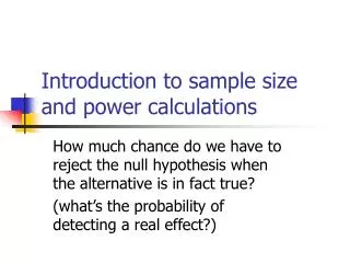
Background • Many quantitative social science research questions are of the form of a hypothesis – A has a significant effect on B. • To answer such a question data is collected that allows the researcher to (hopefully) test whether statistically A has a significant effect on B. (In fact we aim to reject the hypothesis that A doesn’t significantly affect B). • A test is performed and either the researcher is happy and A indeed has a significant effect on B or is left wondering why the data collected do not back up their hypothesis. Is the hypothesis false or was the data not sufficient? • The sufficiency of the data is the motivation for sample size calculations.
Example • Suppose I have the research question ‘Are Welshmen on average taller than 175 cms?’ • I now need to get hold of a random sample of n Welshmen and measure each of their heights. • I make some statistical assumption about the distribution of the heights of Welshmen e.g. that they come from a Normal distribution. • I might like to check this assumption by plotting a histogram of the data. • I can then form a statistical hypothesis test and test whether indeed Welshmen are taller than 175cms. • I need to decide how big to make n, my sample of Welshmen.
Hypothesis Testing • Let us assume our null hypothesis is that the average height of Welshmen (μ) is 175cm. • So we test H0:μ=175 vs HA:μ>175 (or alternatively H0:θ=0 vs HA:θ>0 where θ=μ-175) • In practice we calculate from our sample its mean ( ) and standard deviation (s2) and use these along with n to form a test statistic which we can compare with the distribution assumed under H0
Type I and Type II errors • No hypothesis test is perfect and there is always the possibility of errors • P(Type I error) = α = significance level or size • P(Type II error) = β, 1-β is the power of the test. • In general we fix α to some value e.g. 0.05, 0.01 then 1-β depends on our sample size.
Example hypothesis test • Let us assume that in reality our sample mean is 180cms and the population standard deviation (sd) is 5cms (known). • We can then form a test statistic as follows: • Note here that for small n and unknown sd we should use a student-t distribution rather than Normal. • For a 1-sided Z test we wish Z= > 1.645 and so we need our sample to be of size 3 to reject H0, using a student-t distribution increases this to 5. (Here α=0.05) • However if the sample mean had been only 176cms then we would need n > (1.645*5)2 = 68 Welshmen to reject H0
Power calculations • Our last slide in some sense is backwards as we cannot get from a given sample mean to choosing a sample size! • What we do instead is use different terminology and play God! • We will choose an ‘effect size’, γ which will represent a guess at the increase in the sample mean for Welshmen. • There then exists an (approximate) formula that links four quantities, size (α), power (1-β), effect size (γ) and sample size (n) • Note that the standard error (SE) of γ is a function of n and σ the population sd which is assumed known. • We can now evaluate one of these quantities conditional on the others e.g. what sample size is required given α,1-β and γ? Here RHS is sum of cases H0 true and H0 false.
Welsh height example Here we have looked at two examples with effect sizes 5 and 1 respectively. Assume σ takes the value 5 and so let us suppose we take a sample of size 25 Welshmen. Then Case 1: 5/(5/√25)=1.645+z1-β,z1-β=3.355 β=0.9996 Case 2: 1/(5/ √25)=1.645+z1-β,z1-β=-0.645 β=0.25946 So here a sample of 25 Welshmen from a population with mean 180cms would almost always result in rejecting H0, but if the population mean is 176cms then only 26% of such samples would be rejected. We can plot curves of how power increases with sample size as shown in the next slide.
Power curve for Welshmen example Here we see the two power curves for the two scenarios:
Extending the idea • The simple formula can be used in many situations and hypothesis tests. • To generalise the idea we assume that γ is an effect size associated with a statistic that we wish to compare with a (null) hypothesized value of 0. • The complication occurs in finding a formula for the standard error for the statistic and relating this formula to the sample size, n. • We will next consider an alternative approach before returning to look at how the above approach extends to multilevel models.
The use of simulation • In reality our (hoped for) research path will be as follows: Construct research question -> Form null hypothesis that we believe false -> Collect appropriate data -> Reject hypothesis therefore proving our research question. • Assuming what we believe in our research question is correct and hence null hypothesis is false we can still be let down by not collecting enough data. • The idea behind using simulation is to simulate the data gathering process (assuming we know the right answer) many times and see how often we can reject the null hypothesis. The percentage of rejected null hypotheses (via simulation) will then estimate power.
Simulation in our example • Consider our Welsh height example case 2 where we believe Welshmen have a mean height of 176cms (and sd = 5cms) and we are testing the hypothesis H0:μ=175cms, and we consider a sample size 25. • Then we generate N samples (e.g. 5000) of size 25, • and for each sample form a lower bound for the confidence interval of the form • . This we compare with the value 175 and the proportion greater than 175 is an estimate of the power of the test. • We can repeat this exercise for different sample sizes and form a power curve.
Power curve comparison Note simulation curve is a good approximation of the theoretical curve although there are some minor (Monte Carlo) errors even with 5000 simulations per sample size.
Advantages/Disadvantages • Theoretical approach is quick when the formula can be derived. • Approximations for more complex situations exist which are equally quick. • Simulation approach generalizes to more situations but is much slower and we may need large numbers of simulations per scenario to get accurate power estimates.
What happens with multilevel data? We will here mainly consider 2-level models and take as our application area education, so we have students nested within schools. When deciding on a sampling scheme we have many choices: • How many schools, N ? • How many pupils per school, nj ? • Should we collect the same size sample from each school ? Our decision will depend on which parameter we wish to estimate in the model.
Education Example • For motivation we considered a two level dataset with exam marks measured for each student in a collection of schools. In fact this dataset exists and has 4915 students in 96 schools. • Our hypothesis of interest is that the exam mark for an average student is > 20 (null hypothesis = 20) which with such a large sample results in the null hypothesis being rejected for our particular data. • If we fit the following multilevel model to the data we get the estimates given: • If we treat these estimates as population values, we are interested in what power for testing our hypothesis results from various combinations of N and nj
Design effect formula • If we assume balance then with n pupils in each of N schools for our simple model (and only this simple model) the following formula holds: • Design effect = 1 + (n-1)ρ where ρ is the intra-class correlation. • So if we know the simple random sample size required for a given power we need to multiply this by the design effect. • For example our data has ρ=16.205/(16.205+139.367)=0.104 • So for schools of size 10 pupils we would need 1+9*0.104=1.94 times as many students (in total) to get the same power. • For this model (and this model only) we could therefore perform our power calculations assuming simple random sampling from a population with variance 155.572 and scale up the sample required based on the design. • So • And for schools of size 10 we require 1.94*338.4=657 pupils which we can round up to 66 schools.
Simulating multilevel designs • The process here is similar to the earlier example except that we need to simulate from a multilevel model and fit the models using MLwiN (Rasbash, Browne et al. 2000). • To this end we will write macro code in the MLwiN macro language to perform the task. • The MLwiN macro language allows datasets to be simulated, models to be set up and run using various algorithms and results collected. • It has the advantage of performing all the operations in one package but programming in the macro language is not for the faint hearted!
Simulation continued • We will perform simulations for schools of 10 pupils where number of schools (N) ranges from 5 to 70. For each N, 5000 datasets are generated. • For each dataset we need to generate 10*N level 1 residuals with variance 139.367, N level 2 residuals with variance 16.205 and add these residuals up correctly with the fixed effect estimate 21.685. • MLwiN has commands to generate random Normally distributed observations but also has a SIMU command which given a model is set up and estimates given will simulate from it directly making life easier. • For each simulated dataset we fit the variance components model using the RIGLS algorithm. For small numbers of level 2 units we may have estimation difficulties but MLwiN has an ERROR 0 command which simply ignores such problems. • Note it is also important to ensure the command BATCH 1 is included else MLwiN may only run RIGLS for 1 iteration for each model!!
Comparison of formula/simulations • The following graph compares the design effect formula to the simulation approach:
Zero variance estimates from RIGLS algorithm • The following graph gives a plot of percentage zero estimates for the level 2 variance against number of level 2 units:
Other sample size issues • There are other reasons why we may be interested in sample size questions in multilevel modelling. • It is often problematic to fit multilevel models when the number of higher level units is small as demonstrated in the last graph. • Also some methods can be biased for small sample sizes. • Note although method comparison is done using a similar approach of generating simulated datasets, here power calculations are not the main aim; that said when performing power calculations parameter bias of methods should be noted as this will result in bias of predicted power. • Browne (1998), Browne and Draper(2006) compare MCMC, RIGLS and IGLS for small sample sizes and continuous responses, and MCMC, MQL and PQL for binary response models. • Maas and Hox (2004) also look at small sample sizes and how robust estimation is to the Normal distributional assumption of the level 2 residuals.
Sampling policy The design effect formula: Design effect = 1 + (n-1)ρ suggests that if we are to sample a fixed (balanced) number of pupils n*N then our best power results when n is smallest i.e. sampling one pupil each from 100 schools is better than sampling 100 pupils from the same school. The effect of sampling policy is most important in scenarios where ρ is large e.g. repeated measures designs. The simulation procedure gives approximately the same power curve and so in this simple example we have an easy to use formula. The reason in practice for sampling several pupils from each school is purely the additional cost incurred in visiting additional schools.
More complex examples – random intercepts and random slopes • We will now look at more complex random effect models with predictor variables. • We will consider the random intercept model • and the random slopes model • We will consider how to extend (approximately) the theoretical approach and also the simulation approach.
PINT – (Bosker,Snijders and Guldemond 1996) • Stands for Power IN Two level designs. • Will work out (approximate) standard errors for parameters in two level models. • Allows arbitrary numbers of fixed parameters and random (at level 2) parameters. • Assumes balance at level 2 i.e. each of N level 2 units contains n level 1 units. • Works out (approximate) standard errors for all fixed parameters in the model given lots of information relevant to the calculation. • For each variable, it’s mean, variance (both within and between higher level units) and covariances (correlations) between variables are required in the calculation. • It differentiates between various types of fixed effect: level 1 variables with and without a random effect, level 2 variables and cross-level interactions. • It can also deal with monetary considerations.
Example problem • We will continue with our educational example but also consider the effect of gender (β1). For a random intercepts model let us assume the true parameter values are β0=20.9, β1= 1.6, σ2u=15, σ2e=135. • We have two hypotheses to test: • Hypothesis 1: boys get on average more than 20 marks (H0: β0=20 vs HA: β0>20) • Hypothesis 2: girls do better on average than boys (H0: β1=0 vs HA: β1>0) • We will also consider the effect of random slopes on the dataset so will have a second model with additionally σ2u0=10, σu01=2, σ2u1=5
PINT input • PINT requires us to input σ2u=15, σ2e=135 and for the gender parameter it’s mean (which corresponds to the probability of being a girl) which we will assume is 0.5. We will assume a Binomial assumption for gender making it’s variance equal to 0.25 (within groups) and assume zero variance between groups. • An alternative might be to assume the between groups variance is 0.025 (p(1-p)/n) for the 10 pupils per school example and the within variance 0.225 which increases the parameter SEs slightly and reduces power. • The simulation approach is far easier to understand as we simply choose a gender at random from a Binomial distribution for each pupil. • We can also easily incorporate features such as single sex schools by giving these a probability of selection and making all students in such a school boys or girls.
Results – Hypothesis 1 Here we see good agreement from approaches. It appears that we need a large dataset to have strong power for this hypothesis.
Results – Hypothesis 2 Here the PinT curve appears to give slightly higher power suggesting that maybe the alternative predictor variances would be more appropriate.
What happens when we include random slopes? • The following table gives power values for β1 for the random intercept model. • Note that pairs of values with the same total N*n have similar powers.
What happens when we include random slopes? • The following table gives power values for β1 for the random slopes model. • Note that pairs of values with the same total N*n now do not have similar powers and larger N is better.
Effect of balance • Here we look at 3 scenarios: balanced, unbalanced, severe unbalanced. • We will consider the variance components model and construct power curves by evaluating each scenario at 4,8,12,…,100 schools. • The balanced case for N schools has 10 pupils per school. • The equivalent unbalanced case has N/2 schools containing 5 pupils, N/4 schools containing 10 pupils and N/4 schools containing 20 pupils. • The severely unbalanced case has N-1 schools only containing 1 pupil and 1 school containing 9N+1 pupils.
Results • Here we see the power curves for the 3 scenarios. Note lower power for unbalanced and strange behaviour for severe unbalance.
Number of zero variances Extremely unbalanced designs are really estimating the effect of the large school instead of the global mean and hence the level 2 variance is often estimated as 0.
Subsampling approach / post-hoc power calculations • We have chosen a parametric approach where, given effect sizes, we simulate datasets prior to any actual data being collected. • An alternative post-data collection non-parameteric approach is to subsample from a large existing dataset and test power calculations on these subsamples. • Such an approach has been investigated by Arshartous (1995) and Mok (1995). • The advantage of this approach is that no distributional assumptions need be made in the dataset generation. • The disadvantage is that post-data power calculations in some sense miss the boat in that we really need the power calculations to guide us in our sampling. However such calculations may be useful for similar future studies.
Bayesian approach • A recent more Bayesian approach is described in Wang and Gelfand (2002). • Here rather than fix an effect size for each unknown parameter the user instead can give a prior distribution (the sampling prior) which is used in the generation of the simulated datasets. • They then use MCMC to fit models to their simulated datasets and evaluate performance criterions based on the posterior samples.
Cross-classified models • In our ESRC grant we are intending to focus on these model types for our Power calculations as they are outside the remit of PINT. • To date we have produced code in both MLwiN (using both the Rasbash and Goldstein adaptation of the IGLS algorithm and MCMC sampling) and R (lmer). • MLwiN appears to be quicker although both lGLS and lmer have problems as the number of units in the cross-classified models increases, particularly with random slopes.
Cross-classified Issues • We have considered 2 higher level classifications and an educational application where pupils are nested in both districts (where they live) and schools (where they study). Districts and schools are crossed. • This data structure can be considered as a 2-way contingency table. • Note that in reality this table will be sparse i.e. a school takes mainly pupils from local districts. • We can consider sampling where we can choose any number from any cell of the table or perhaps more realistically we could choose numbers of pupils from one dimension e.g. school and simply be given their district from sampling. • For simulation purposes we can create typical tables based on probabilities of cell membership. • We plan to compare approaches to mimic the sampling process.
Conclusions • In this talk we have shown the flexibility of using simulation to perform power calculations for multilevel models. • Although computationally the approach is slow the flexibility of the approach means it can be used for virtually all models given enough assumptions. • Low powered studies often involve small amounts of data thus making the power calculations quicker. • In comparison the PINT program is fantastically quick and it will be worth also using the simulation approach to make approximate adjustments to PINT answers for problems it cannot deal with.
Further work: Designing a Power simulator software package • We are interested in using MLwiN (both IGLS and MCMC estimation), lmer in R and WinBUGS for fitting models to simulated datasets. • We want a stand-alone program that generates macro code to be run in either MLwiN, Winbugs or R. • The idea is the program takes as input details of the model to be investigated and generates code for the problem that can be used in the appropriate software package.
Further work • Find (faster) approximations to simulation results – potentially create look up tables, power curves etc. • Investigate other packages for power calculations e.g. optimal design (Raudenbush et al. 2005) for cluster randomized trials. • Investigate the Bayesian approach of Wang and Gelfand (2002) and compare with the standard approach. • Investigate efficient MCMC methods. • Investigate models with other response types.
References • Arshartous, D. (1995). Determination of Sample Sizes for Multilevel Model Design. Multilevel Analysis for Education Research. • Bosker, R.J., Snijders, T.A.B. and Guldemond, H. (1996) PINT (Power IN Two-level designs) User Manual. • Browne, W.J. (1998) Applying MCMC methods to Multi-level models. Unpublished PhD. thesis. University of Bath. • Browne, W.J. and Draper, D. (2006) A comparison of Bayesian and likelihood-based methods for fitting multilevel models (with discussion). Bayesian Analysis1, 473-550. • Mass, C.J.M. and Hox, J.J. (2004) Robustness issues in multilevel regression analysis. Statistica Neerlandica58, 127-137. • Mok, M. (1995) Sample Size Requirements for 2-level Designs in Educational Research. Multilevel Modelling Newsletter7 (2): 11-15 • Rasbash, J, Browne, W.J., Goldstein, H. et al. (2000). A User’s Guide to MLwiN version 2.1, London: Institute of Education, University of London. • Wang, F. and Gelfand, A.E. (2002) A simulation-based approach to Bayesian sample size determination for performance under a given model and for separating models. Statistical Science17 (2): 193-208.