Modeling Continuous Variables
E N D
Presentation Transcript
Modeling Continuous Variables Lecture 19 Section 6.1 - 6.3.1 Tue, Feb 19, 2008
Models • Mathematical model – An abstraction and, therefore, a simplification of a real situation, one that retains the essential features. • Real situations are usually much to complicated to deal with in all their details.
Example • The “bell curve” is a model (an abstraction) of many populations. • Real populations have all sorts of bumps and twists and irregularities. • The bell curve is smooth and perfectly symmetric. • In statistics, the bell curve is called the normal curve, or normal distribution.
Models • Our models will be models of distributions, presented either as histograms or as continuous distributions.
Histograms and Area • In a histogram, frequency is represented by area. • Consider the following distribution of test scores.
Frequency 10 8 6 4 2 Grade 0 70 80 90 60 100 Histograms and Area
Histograms and Area • What is the total area of this histogram?
Frequency 10 90 8 80 6 50 4 30 2 Grade 0 70 80 90 60 100 Histograms and Area
Histograms and Probability • If we selected one student at random, what is the probability that he earned a grade between 70 and 79?
Histograms and Area • We will rescale the vertical axis so that the total area equals 1, representing 100%.
Histograms and Area • To achieve this, we divide the frequencies by the original area to get the density.
Histograms and Area Density 0.040 0.030 0.020 0.010 Grade 0 70 80 90 60 100
Histograms and Area Density 0.040 0.36 0.030 0.32 0.020 0.20 0.010 0.12 Grade 0 70 80 90 60 100
Histograms and Area Density 0.040 Total area = 1 0.36 0.030 0.32 0.020 0.20 0.010 0.12 Grade 0 70 80 90 60 100
Histograms and Area • This histogram has the special property that the proportion can be found by computing the area of the rectangle. • For example, what proportion of the grades are less than 80? • Area = 0.12 + 0.32 = 0.44 = 44%.
Density Functions • This is the fundamental property that connects the graph of a continuous model to the population that it represents, namely: • The area under the graph between two points on the x-axis represents the proportion of the population that lies between those two points.
Density Functions AREA = PROPORTION = PROBABILITY
x Density Functions • Consider an arbitrary continuous distribution.
x a b Density Functions • The area under the curve between a and b is the proportion of the values of x that lie between a and b.
x a b Density Functions • The area under the curve between a and b is the proportion of the values of x that lie between a and b.
x a b Area = Proportion Density Functions • The area under the curve between a and b is the proportion of the values of x that lie between a and b.
x a b Area = Probability Density Functions • The area also represents the probability that a randomly selected value of x will lie between a and b.
x a b Density Functions • The total area under the curve must be 1, representing a proportion of 100%.
100% x a b Density Functions • The total area under the curve must be 1, representing a proportion of 100%.
The Normal Distribution • Normal distribution – The statistician’s name for the bell curve. • It is a density function in the shape of a “bell.” • Symmetric. • Unimodal. • Extends over the entire real line (no endpoints). • “Main part” lies within 3 of the mean.
The Normal Distribution • The curve has a bell shape, with infinitely long tails in both directions.
The Normal Distribution • The mean is located in the center, at the peak.
The Normal Distribution • The width of the “main” part of the curve is 6 standard deviations wide (3 standard deviations each way from the mean). + 3 – 3
The Normal Distribution • The area under the entire curve is 1. • (The area outside of 3 st. dev. is approx. 0.0027.) Area = 1 + 3 – 3
The Normal Distribution • The normal distribution with mean and standard deviation is denoted N(, ). • For example, if X is a variable whose distribution is normal with mean 30 and standard deviation 5, then we say that “X is N(30, 5).”
The Normal Distribution • If X is N(30, 5), then the distribution of X looks like this: 15 30 45
Some Normal Distributions • NormalDistributions.nb
Some Normal Distributions N(3, 1) 6 5 4 7 8 3 2 1 0
N(5, 1) Some Normal Distributions N(3, 1) 6 5 4 7 8 3 2 1 0
Some Normal Distributions N(2, ½) N(5, 1) N(3, 1) 6 5 4 7 8 3 2 1 0
Some Normal Distributions N(2, ½) N(3½, 1½) N(5, 1) N(3, 1) 6 5 4 7 8 3 2 1 0
