Download
1 / 18
190 likes | 316 Views
Learn about the crucial factors influencing the Bragg peak in proton beam therapy design, including range modulation, nuclear interactions, and dosimeter calibration. Explore how beam energy affects peak shape and how nonelastic nuclear reactions impact dose distribution.

E N D
Bragg Peak The Bragg peak, as we use the term, is the on-axis depth-dose distribution, in water, of a broad quasi-monoenergetic proton beam. A carefully measured Bragg peak is essential to accurate range modulator design. Listing the most important factor first, the shape of the Bragg peak depends on the fundamental variation of stopping power with energy, the transverse size of the beam, range straggling, beam energy spread, nuclear interactions, low energy contamination, effective source distance, and the dosimeter used in the measurement. Because of range straggling, the peak of the depth-dose distribution increases in absolute width as beam energy increases. Usually, the Bragg peak is measured with an uncalibrated dosimeter. In other words, x values (depth in water) are known absolutely and rather accurately but y values (dose) are relative. To prepare such a measured Bragg peak for use in design programs we fit it with a cubic spline, correct for the fluence at measurement time, and convert y to absolute units, Gy/(gp/cm2). The last step, renormalization, allows subsequent calculations to yield absolute dose estimates.
3 2 i = 1 (S/ρ)1Φ22N2 Motivation This figure shows schematically how we design a range modulator by adding appropriately weighted Bragg peaks. To be successful we need to measure the Bragg peak accurately and under the correct conditions.
Anatomy of the Bragg Peak 1/r2 and transverse size set peak to entrance ratio the dosimeter matters overall shape from increase of dE/dx as proton slows width from range straggling and beam energy spread nuclear buildup or low energy contamination this part is a guess nuclear reactions take away from the peak and add to this region depth from beam energy
Anatomy of the Bragg Peak in Words 1. The increase of dE/dx as the proton slows down causes the overall upwards sweep. 2. The depth of penetration (measured by d80 ) increases with beam energy. 3. The width of the peak is the quadratic sum of range straggling and beam energy spread. 4. The overall shape depends on the beam’s transverse size. Use a broad beam. 5. Non-elastic nuclear reactions move dose from the peak upstream. 6. A short effective source distance reduces the peak/entrance ratio. Be sure you know and record your source distance. 7. Low energy beam contamination (as from collimator scatter) may affect the entrance region. Use an open beam. 8. The exact shape depends somewhat on the dosimeter used. Use the same dosimeter you plan to use later in QA.
Effect of Nonelastic Nuclear Reactions This figure is a Monte Carlo calculation by Martin Berger (NISTIR 5226 (1993)). Dashed line: nuclear reactions switched off; solid line: actual BP. Buildup, not usually a problem because of the likely presence of buildup material near the patient, is ignored. Dose from the EM peak shifts upstream, lowering the peak and flattening the entrance region, especially at high proton energies. Because nuclear reactions are hard to model, we take them into account by using a measured (rather than predicted) Bragg peak to deduce an effective stopping power which includes nuclear reactions.
Nuclear Buildup The ‘local energy deposition’ approximation fails at the entrance to a water tank where longitudinal equilibrium has not yet been reached. You can see this if you measure a Bragg peak vertically so that the proton beam enters from air. This scan, courtesy of IBA, is from the Burr Center. An excellent early paper is Carlsson and Carlsson, ‘Proton dosimetry with 185 MeV protons: dose buildup from secondary protons and recoil electrons,’ Health Physics 33 (1977) 481-484. It also discusses the (much more rapid) electron buildup. Observed nuclear buildup is smaller than one would expect; that has not been explained so far. A therapy beam usually has buildup material near the patient, so the effect shown above can be ignored.
Bragg Peak Shape vs. Beam Energy Bragg peaks from 69 to 231 MeV (courtesy IBA) normalized so the entrance value equals the tabulated dE/dx at that energy. Straggling width relative to range is almost independent of energy so absolute straggling width increases with energy. Therefore the Bragg peak gets wider. The change in shape makes active range modulation more complicated than passive, where we simply ‘pull back’ a constant shape.
Transverse Equilibrium The fluence on the central axis of a pencil beam decreases with depth because of out-scattering of the protons. The dose on axis (fluence × stopping power) therefore goes down; the Bragg peak vanishes. A scan along the axis with a small ion chamber would show this; a scan with a large one would not. In a broad beam the axial fluence is restored by in-scattering from neighboring pencils (transverse equilibrium). A scan along the axis with a small ion chamber will therefore measure the ‘true’ Bragg peak. It is essential to use this ‘broad beam’ geometry if we wish to use the measured Bragg peak to design range modulators.
Transverse Equilibrium (Theory) Behavior of the Bragg peak as the beam cross section is made smaller : W.M. Preston and A.M. Koehler, ‘The effects of scattering on small protons beams,’ unpublished manuscript (1968) Harvard Cyclotron Lab, available on BG Web site.
Transverse Equilibrium (Experiment) Hong et al. ‘A pencil beam algorithm for proton dose calculations,’ Phys. Med. Biol. 41 (1996) 1305-1330. Also shows low energy contamination by collimator-scattered protons.
Dosimeter Response (left) from H. Bichsel, ‘Calculated Bragg curves for ionization chambers of different shapes,’ Med. Phys. 22 (1995) 1721. He compares the response of an ideal (‘point’) IC, a plane-parallel IC (less peaked) and an exaggerated thimble IC (much less peaked). The effect is geometric: the thimble samples protons with a spread of residual ranges. (right) from A.M. Koehler, ‘Dosimetry of proton beam using small silicon diodes,’ Rad. Res. Suppl. 7 (1967) 53. Response is ≈8% higher than a PPIC in the Bragg peak for the diode (long obsolete) used by Andy. Not all diodes behave this way. A diode marketed by Scanditronix specifically for radiation dosimetry behaves very like a PPIC.
Tips for Measuring the Bragg Peak • When you measure Bragg peaks for later use in modulator design: • Use a broad beam (several cm). Check by moving axis. • Use an open nozzle to avoid low-energy contamination. • Know and record the effective source distance. • Know and record the beam spreading system. • Know and record tank wall thickness and other depth corrections. • If beam energy spread is adjustable, use the clinical setting. • Use the same dosimeter as you plan to use for clinical QA.
Preparing the Bragg Peak for Use Fit data with a cubic spline (BPW.FOR) to put the Bragg peak in a compact standard form (e.g. IBA231.BPK). That also averages out the experimental noise. Extrapolate to 0 cm H2O if desired. Later, open the BPK file with: CALL InitBragg(t1,0.,bl,x1,xl,xp,xh,xm,'\BGware\DATA\'//bf) which does the following: • stretches the peak (if desired) so d80 = xh corresponds to t1 • divides by fluence (1/r2) to yield an effective stopping power • normalizes so entrance dE/dx = tabulated EM value • returns various parameters of interest (xp, xh ...) Subsequently, y = Bragg(x) will return the effective mass stopping power S/ρ (Gy/(gp/cm2)) at depth x. On using the formula D = Φ (S/ρ) = fluence × mass stopping power the design program will get the absolute dose rate automatically.
Model Independent Fit with Cubic Spline Measured Bragg peak (courtesy IUCF) fit with a cubic spline (open squares). See the description of BPW.FOR in the NEU User Guide NEU.PDF . This step puts the Bragg peak in a compact standard form and averages over experimental noise.
Output File from Fitting Program BPW A standard Bragg peak (.BPK) text file consisting of an array of depths and a corresponding array of relative dose points. The program that opens this file uses the effective source distance to compute the relative fluence (1/r2) at Bragg measurement time and correct for it. It also renormalizes the dose values so the entrance dose corresponds to tabulated dE/dx, obtaining an absolute effective mass stopping power expressed in Gy/(gp/cm2).
The Effective Mass Stopping Power The Bragg peak is a depth-dose distribution taken under specific conditions. Beam line design programs, generally speaking, compute proton fluence from multiple scattering theory and need to use dose = fluence × stopping power to compute the dose. Therefore we would like to derive from the measured Bragg peak an effective mass stopping power (a function of equivalent depth in water) for that particular cohort of protons. To do this we use the fundamental equation to define d is depth in water, D(d) is the BP measurement and Φ(d) is the fluence at BP measurement time. That can be approximated by 1/r2 if we know the source distance. To distinguish the effective stopping power from tabulated stopping powers we assign it the units Gy/(gp/cm2) (gp ≡ 109 protons). The effective stopping power includes nuclear reactions, energy straggling, beam energy spread and all other effects relevant to range modulator design. If you want, you can just think of it as the Bragg peak corrected for 1/r2 at measurement time to bring it into a standard form.
Renormalizing the Bragg Peak So far we only know the relative value of (S/ρ)eff : its shape as a function of d. If we could somehow assign a rough absolute value to it our design program would automatically predict the dose per incident (109) protons (gp) in a given beam line. One way of doing this is to assume that the rate of energy loss at the BP entrance point corresponds to the tabulated EM dE/dx at the incident energy T1. Performing the required conversions we find that we should set Gy/(gp/cm2) where S/ρ on the RHS is the tabulated EM stopping power in MeV/(g/cm2). The flaw in that reasoning is that, if the BP is measured under conditions of longitudinal (nuclear) equilibrium, the dE/dx we assign to the entrance point should also include a contribution from nuclear secondaries, a ≈10% effect. Because of the uncertainty in the nuclear part (see Carlsson and Carlsson) we simply ignore it for now. Alternatively, we might have renormalized S/ρ using the fact that the area under the BP corresponds to T1. The flaw in that reasoning is that, while the average proton certainly brings in T1 , it doesn’t deposit T1 in the water. A few percent (depending on T1) is carried off by neutrons and photons. The tension between ‘entrance’ and ‘area’ normalization is discussed in extenso in our book. Since we only use it for dose-per- proton estimates (never to determine the treatment dose) it doesn’t matter that much.
Summary We certainly understand the underlying physics (which we have outlined) of the Bragg peak. In the past, the Bragg peak has been modeled numerically (Bichsel), by Monte Carlo calculations (Berger, Seltzer and many others) and even analytically (Bortfeld, Med. Phys. 24 (1997) 2024-2033). However, each of these methods requires parameters that are not known a priori at a given accelerator and beam line. They are, at a minimum, the exact range, the beam energy spread, and a parameter characterizing low energy contamination or inelastic nuclear reactions. In other words one cannot, without the aid of measurements, compute entirely from first principles a Bragg peak accurate enough for modulator design. For that reason we favor a direct model-independent characterization of the data by means of a cubic spline fit. We have listed precautions to be observed when obtaining the data. We have also described how we prepare Bragg peak data for use in beam line design programs, especially with a view to range modulator design. We fit the data with a cubic spline, correct them for 1/r2 (the fluence at Bragg measurement time) and renormalize them to create a function Bragg(depth) which can be used as an effective mass stopping power for the relevant cohort of protons. Because it is based on direct measurements it automatically includes all such effects as beam energy width and nonelastic reactions.