Metabolomics
Metabolomics. PCB 5530 Tom Niehaus Fall 2012. Definitions and Background. Metabolome = the total metabolite pool. - All low molecular weight (MW < 1000 Da) organic molecules in a sample such as a leaf, fruit, or tuber. Peptides Oligonucleotides Sugars Nucleosides Organic acids


Metabolomics
E N D
Presentation Transcript
Metabolomics PCB 5530 Tom Niehaus Fall 2012
Definitions and Background Metabolome = the total metabolite pool - All low molecular weight (MW < 1000 Da) organic molecules in a sample such as a leaf, fruit, or tuber. Peptides Oligonucleotides Sugars Nucleosides Organic acids Ketones Aldehydes Amines Amino acids Lipids Steroids Alkaloids Drugs (xenobiotics)
Definitions and Background Metabolomics = high-throughput analysis of metabolites Metabolomics is the simultaneous ('multiparallel') measurement of the levels of a large number of cellular metabolites (typically several hundred). Many of these are not identified (i.e. are just peaks in a profile).
Definitions and Background Metabolomics = high-throughput analysis of metabolites Metabolomics analysis is like a snapshot, showing which compounds are present and at what relative levels at a specific time point. More generally, metabolomics refers to a holistic analytical approach to metabolism that is not guided by specific hypotheses. Instead, metabolomics sets out to determine how (in principle, all) metabolite levels respond to genetic or environmental changes and, from the data, to generate new hypotheses.
Definitions and Background Fluxomics = A branch of metabolomics that measures the turnover of metabolites in pathways using labeled isotopes such as 13C. - New technology, just beginning to be utilized - Instead of being a snapshot of metabolism, it is like a movie
Definitions and Background History and Development Metabolic profiling is not new. Profiling for clinical detection of human disease using blood and urine samples has been carried out for Centuries. This urine wheel was published in 1506 by UllrichPinder, in his book EpiphanieMedicorum. The wheel describes the possible colors, smells and tastes of urine, and uses them to diagnose disease. Nicholson, J. K. & Lindon, J. C. Nature 455, 1054–1056 (2008).
Definitions and Background History and Development Advanced chromatographic separation techniques were developed in the late 1960’s. Linus Pauling published “Quantitative Analysis of Urine Vapor and Breath by Gas-Liquid Partition Chromatography” in 1971 Chuck Sweeley at MSU helped pioneer metabolic profiling using gas chromatography/ mass spectrometry (GC-MS) Gates SC, Sweeley CC (1978) Quantitative metabolic profiling based on gas chromatography. ClinChem 24:1663-73. Quantitative metabolic profiles of volatilizable components of human biological fluids, e.g. urinary organic acids, were established using GC/MS. Data were processed by computer and statistical methods for analyzing metabolic profiles were developed. [Note that all the elements of metabolic profiling are here.]
Definitions and Background History and Development Plant metabolic biochemists (e.g. LotharWillmitzer) were among other early leaders in the field. Metabolomics is expanding to catch up with other multiparallel analytical techniques (transcriptomics, proteomics) but remains far less developed and less accessible.
Definitions and Background Plant Metabolome Size It is estimated that all plant species contain 90,000 - 200,000 compounds. Each individual plant species contains about 5,000 – 30,000 compounds. e.g. ~ 5,000 in Arabidopsis The plant metabolome is much larger than that of yeast, where there are far fewer metabolites than genes or proteins (<600 metabolites vs. 6000 genes). The size of the plant metabolome reflects the vast array of plant secondary compounds. This makes metabolic profiling in plants much harder than in other organisms.
Definitions and Background Metabolomics compared to Genomics, Transcriptomics, and Proteomics Differences between metabolomics and the other multiparallel approaches: 1 GENE → 1 mRNA → 1 Protein → Many Metabolites (and conversely: Many proteins → 1 Metabolite) (a) Conceptual: There is no direct relationship between metabolite and gene in the way there is between genes and mRNAs and proteins. A single gene does not specify the level of a single metabolite, i.e. its pool size (although it may determine whether the metabolite is present or absent). Rather, as MCA teaches, the level of a metabolite is determined by the activities of all the enzymes of all the pathways that involve that metabolite, and by effectors that act on these enzymes. In practice, therefore, metabolite levels change according to developmental, physiological, and pathological states. Biological variance in metabolite levels (i.e., the variation between genetically identical plants grown in the same conditions) is accordingly large – about 10× the analytical variability – and limits the resolution of metabolomics.
Definitions and Background Metabolomics compared to Genomics, Transcriptomics, and Proteomics Differences between metabolomics and the other multiparallel approaches: (b) Chemical: Unlike nucleic acids and proteins, metabolites have a vast range of chemical structures and properties. Their molecular weights span two orders of magnitude (30–3000 Da). Therefore no single extraction or analysis method works for all metabolites. (Unlike DNA sequencing, microarrays, MS analysis of proteins – all are general methods.) (c) Dyamic: Many metabolite levels change with half times of minutes or seconds – far faster than nucleic acids or proteins. Thus valuable information is lost if sampling times are too far apart. Also drastic artifactual changes can occur in short intervals between harvest and extraction; this adds to biological variance.
Definitions and Background The Power of Metabolomics Metabolomics analysis can powerfully complement transcriptomics and proteomics. Metabolomes are a step nearer actual function. Transcriptomes or proteomes are very inadequate monitors of cell function because there is no simple relationship between mRNA or protein levels and metabolism. Thus changes in mRNA level or protein level in mutants or transgenics are usually not closely linked to changes in metabolic function or phenotype as a whole. Part of the reason for this is the non-linear relation between mRNA and protein levels (see graph) and the typically hyperbolic relation between enzyme level and in vivo flux rate (see MCA class). Another cause is the high level of functional redundancy in plant metabolism – i.e. parallel or alternative pathways for the same process. The dependence of protein expression on mRNA levels, in linear coordinates. PMID: 1718905
Definitions and Background The Power of Metabolomics Silent Knockout Mutations. ~90% of Arabidopsis knockout mutations are silent – i.e. have no visible phenotype and so provide no clues to gene function. (The search for some sort of visible phenotype therefore often becomes desperate.) The situation in yeast is similar – up to 85% of yeast genes are not needed for survival. When there is little or no change in growth rate (visible phenotype) of a knockout mutant, the pool sizes of metabolites have altered so as to compensate for the effect of the mutation, leaving metabolic fluxes are unchanged. Thus – intuitively – mutations that are silent when scored for metabolic fluxes or growth rate (growth rate is the sum of all metabolic fluxes) should have obvious effects on metabolite levels. There is a firm theoretical basis for this in MCA.
Definitions and Background The Power of Metabolomics Example. In the Chloroplast 2010 project (phenotype analysis of knockouts of Arabidopsis genes encoding predicted chloroplast proteins): Various knockouts showed essentially normal growth and color but highly abnormal free amino acid profiles, e.g. At1g50770 (‘Aminotransferase-like’)
Metabolic Profiling Methods Sample Preparation Metabolites are typically extracted in aqueous or methanolic media, then fractionated into lipophilic and polar phases that are then analyzed separately. Further fractionation of each phase may follow to split metabolites into classes prior to analysis. No single extraction procedure works for all metabolites because conditions that stabilize one type of compound will destroy other types or interfere with their analysis. Therefore the extraction protocol has to be tailored to the metabolites to be profiled.
Metabolic Profiling Methods Sample Preparation In practice, these considerations mean that metabolic profiling is often confined to fairly stable compounds that can be extracted together. These include major primary metabolites (sugars, sugar phosphates, amino acids, and organic acids) and certain secondary metabolites (e.g., phenylpropanoids, alkaloids). The most comprehensive profiling can cover several hundred such compounds, many of which are unidentified. Many crucial metabolites, particularly minor or unstable ones, are currently being missed in metabolomics analyses.
Metabolic Profiling Methods Main Analytical Techniques Gas Chromatography/Mass-Spectrometry (GC/MS) In GC/MS, it may be necessary to first derivatize the sample to increase metabolite stability and volatility. The derivatized mix is then fractionated by a gas chromatograph that is coupled to a mass spectrometer. The mass spectrometer scans the peaks emerging from the GC column at frequent intervals (~1 sec) and so acquires the mass spectrum of each peak, from which peaks can be identified and quantified. Mass spectrometry ‘weighs’ ionized individual molecules and their fragments. Molecules are identified from their fragmentation pattern and ‘weights’ (mass/charge ratios – m/z values), with the help of mass spectra libraries, and can be quantified from peak size.
Metabolic Profiling Methods Main Analytical Techniques Gas Chromatography/Mass-Spectrometry (GC/MS) Overlapping peaks can be deconvoluted because the spectra of their constituents are distinct Target metabolites are identified by exact retention times and their corresponding mass spectra (B) as shown for the co-eluting peaks of malate, gamma-aminobutyric acid (GABA), and an unidentified compound. m/z, Ratio of mass to charge. PMID: 11062433
Metabolic Profiling Methods Main Analytical Techniques Gas Chromatography/Mass-Spectrometry (GC/MS) Unfortunately, knowing only the exact masses of molecules and their fragments is not enough to identify them. Huge number of chemical structures can have the same exact mass. This is why libraries of retention times and mass spectra, determined for standard compounds, are critical. The major challenge for metabolomics is identification of unknown peaks. Basically, standards are essential to the process. If there is no standard, a compound cannot be identified with certainty. Thus, the more novel the compound, the less powerful metabolomics becomes. Mass spectrometry (MS) metabolomic datasets provide relative quantification of cellular metabolites (i.e. –fold changes in levels between different samples. Absolute quantification (i.e. moles per weight of tissue) is possible with MS methods but requires an authentic standard for each metabolite to be quantified. Animated explanation of GC/MS: http://www.shsu.edu/~chm_tgc/sounds/flashfiles/GC-MS.swf Tutorial on MS: http://www.asms.org/whatisms/page_index.html
Metabolic Profiling Methods Main Analytical Techniques Liquid Chromatography/Mass-Spectrometry (LC/MS) In LC/MS (also termed high performance liquid chromatography, HPLC/MS) the samples are not derivatized before analysis and an HPLC instrument is used for separation. LC/MS is more suitable than GC/MS for labile compounds, for those that are hard to derivatize, or hard to render volatile. LC/MS is less developed than GC/MS. A closely related method is capillary electrophoresis (CE)/MS.
Metabolic Profiling Methods Main Analytical Techniques PMID: 11553758 Liquid Chromatography/Mass-Spectrometry (LC/MS) Profiling example: Metabolites related to plant isoprenoid biosynthesis. The total ion chromatogram (TIC) is the total output of the ion detector; the extracted ion chromatograms (EICs) are the outputs for particular ions characteristic of isoprenoid synthesis intermediates. LC-MS analysis of endogenous pools of prenyldiphosphates in isolated peppermint oil gland secretory cells. A, Total ion chromatogram (TIC; m/z 50–350) B, detection of endogenous GPP in the m/z 313 [(M − H)−] extracted ion chromatogram (EIC) C, detection of endogenous DMAPP and IPP in the m/z 245 [(M − H)−] EIC D, EIC of a mixture of authentic DMAPP and IPP standards at m/z 245 [(M − H)−].
Metabolic Profiling Methods Main Analytical Techniques Nuclear Magnetic Resonance (NMR) Spectroscopy Advantages of NMR over MS: - NMR does not destroy the sample - NMR can detect and quantify metabolite because the signal intensity is only determined by the molar concentration - NMR can provide comprehensive structural information, including stereochemistry Many atoms have nuclei that are NMR active, but most NMR data are collected for 1H and 13C since these are present in all organic molecules. The main weakness of NMR is low sensitivity relative to MS. It is therefore less suited for analysis of trace compounds. As the natural abundance of 13C is only 1.1%, 13C-NMR is less sensitive than 1H-NMR. Recent developments have considerably increased sensitivity, making it less of a problem.
Metabolic Profiling Methods Main Analytical Techniques Nuclear Magnetic Resonance (NMR) Spectroscopy NMR uses radio-frequency (RF) radiation and magnetic fields. RF radiation is used to stimulate nuclei present within molecules. The information obtained is displayed as a spectrum. The horizontal axis is the chemical shift (delta, in units of ppm), which is a measure of the position at which RF absorption occurs relative to an internal standard (tetramethylsilane, TMS). The vertical axis is the intensity of the absorption. As with other spectral techniques, compounds have characteristic spectra. More than 100 metabolites occur in plants at levels high enough for analysis by NMR, so NMR spectra of mixtures contain many peaks.
Metabolic Profiling Methods Main Analytical Techniques Nuclear Magnetic Resonance (NMR) Spectroscopy Profiling example: 1H-NMR spectra of extracts of leaves of various Verbascum species (medicinal plants) 600 MHz 1H NMR spectra of extracts of Verbascum leaves. From bottom to top: V. xanthophoeniceum, V. nigrum, V. phlomoides, V. phoeniceum, V. phlomoides, V. densiflorum. PMID: 21807390
Metabolic Profiling Methods Main Analytical Techniques Nuclear Magnetic Resonance (NMR) Spectroscopy Signal overlap is a problem in the complex spectra of plant extracts. Signal overlap hampers metabolite identification and quantification. Better signal resolution can be obtained using various types of 2D NMR spectroscopy. These approaches cut signal overlap by spreading the resonances in a second dimension. Example: Heteronuclear single quantum coherence (HSQC) spectroscopy. The 2D spectrum has one axis for 1H and the other for a heteronucleus (an atomic nucleus other than a proton), usually 13C or 15N. The spectrum contains a peak for each unique proton attached to the heteronucleus being considered. NMR tutorial: http://www.cis.rit.edu/htbooks/nmr/
Metabolic Profiling Methods Main Analytical Techniques Nuclear Magnetic Resonance (NMR) Spectroscopy HSQC used to select for protons directly bonded to 13C. Use of HSQC spectroscopy for analysis of common metabolites. In 1D spectra, overlapped signals hamper identification of individual metabolites, whereas in 2D correlation, spots are easily visible. (a) 1D 1H NMR spectrum of an equimolar mixture of the 26 standards. (b) 2D 1H–13C HSQC NMR spectra of the same synthetic mixture (red) overlaid onto a spectrum of aqueous whole-plant extract from Arabidopsis (blue). PMID: 21435731
Metabolic Profiling Methods Main Analytical Techniques How can one decide which analytical platform should be used? - Should be rapid, reproducible, with easy sample preparation. - Selection based on objectives, target metabolites, availability, etc. Scale from - to +++ for major disadvantages to major advantages Phytochem Rev (2008) 7:525–537
Data Analysis The avalanche of metabolome data presents great difficulties to analyze. There are also challenges in archiving such data; a standard framework for this is in place. The problems in extracting meaning from large data sets are similar for all forms of profiling. The goal is to recognize patterns for further exploration. Various data mining tools are used for this. These statistical tools reduce data complexity by focusing on the information content of a given data set, i.e. they try to ‘tame’ the wild profusion of profiling data. Unlike many other statistical procedures, these methods are mostly applied when there are no a priori hypotheses. Data mining tools include cluster analysis (CA) and principal components analysis (PCA). The metabolite data can be known or unidentified peaks. CA and PCA can establish ‘guilt by association’ – they can point to where in metabolism mutations act from the similarity of their metabolite profiles to those of known mutations. External factors (e.g. toxins, herbicides, environmental insults) can be studied in an analogous way.
Data Analysis Thus, in principle, the function of an unknown gene can be determined by comparing the metabolic profile of a mutant in that gene with a library of such profiles generated by deleting individual genes of known function. Caution: This approach may not be so useful for dissecting metabolic responses to normal environmental variations (e.g. in nutrient level, soil aeration, salinity, water supply). There is good reason from MCA theory and from observation to expect such variations to cause relatively little change in metabolite levels. This is because all enzymes in affected pathways tend to be up- or down-regulated together (Fell, 2005). Two key drawbacks of clustering and other current data mining methods are: - Typically, they detect only simple, one-to-one linear relationships. They do not detect non-linear or multi-input relationships, which are common in biology. - They do not assign confidence levels, so it is not clear which clusters are trustworthy when the input data are not well separated.
Data Analysis Cluster Analysis (CA) CA is a set of statistical methods that group similar data together. The group (‘cluster’) members have certain properties in common and the resultant classification can yield new insights. The classification reduces the dimensionality of a data set. Data are presented in dendrograms that emphasize natural groupings.
Data Analysis Cluster Analysis (CA) Profiling example: Dendrogramof the metabolic profiles of transgenic potato tubers and tubers incubated in a range of glucose concentrations (0 to 500 mM). Note that: 1) The glucose-fed samples form a cluster that is nearer the cluster of wild-type samples than any of the transgenics. 2) That independent transgenic lines carrying the same transgene (e.g., the four ‘SP’ lines) tend to cluster together (the principle of ‘guilt by association’). Transgenic lines Dendogram obtained after CA of the metabolic profiles of genetically and environmentally modified potato tuber tissue. PMID: 11158526
Data Analysis Principal Component Analysis (PCA) PCA uses all the metabolite data from a sample to compute an individual metabolic profile that is then compared to all the other profiles. In essence, PCA takes the resulting cloud of data points and rotates it such that the maximum variability is visible – i.e. the extraction of principal components amounts to a variance maximizing rotation of the original variable space. PCA finds the vectors (‘principal components’) that give the best overall sample separation. The data can be represented as two- or three-dimensional plots in which the axes (principal components or vectors) are those that include as much as possible of the total information derived from metabolic variances.
Data Analysis Principal Component Analysis (PCA) Profiling example: Clusters found after PCA analysis of the same data set for potato tubers as above. Note that: 1) The two components chosen account together for 69% of the total metabolic variance, i.e. only 1/3 of the original variation has been lost during data reduction. 2) As before, the glucose-fed samples form a cluster that is nearer the cluster of wild-type samples than any of the transgenics. 3) Again, independent transgenic lines carrying the same transgene (e.g., the four ‘SP’ lines) tend to cluster together. PCA of the metabolic profiles of genetically and environmentally modified potato tuber tissue. PMID: 11158526
Data Analysis Simple Correlations Computer-generated pairwise plots of every metabolite in the data set against every other metabolite can be informative. But when hundreds of metabolites are analyzed the potential number of such plots is very large – many thousands – and most of them will show no relationship.
Data Analysis Simple Correlations Profiling examples: correlations between pairs of metabolites among transgenic potato tubers. Note: 1) The linear correlation (Frame A) between glucose-6-phosphate and fructose-6-phosphate levels. These metabolites are interconvertible by phosphoglucoseisomerase, which catalyzes a near-equilibrium reaction. A linear relation is thus predicted. 2) The non-linear correlation between methionine and lysine levels (Frame C), in which lysine accumulates continuously but methionine reaches a plateau. This is expected because methionine synthesis is under tighter feedback and feedforward control than lysine. Correlation between metabolite levels of the transgenic potato tissues. PMID: 11158526
Metabolomics Resources http://fiehnlab.ucdavis.edu/Oliver Fiehn’s group at UC Davis. Includes databases. http://www.noble.org/plantbio/MS/metabolomics.html Lloyd Sumner’s group at the Noble Foundation. Useful short summary of analytical approaches and bioinformatics involved in metabolomics. http://dbkgroup.org/default.htmDouglas Kell’s group at University of Manchester – a gateway site with explanations of metabolic profiling technologies and links to other useful sites.
Useful Values (for interpreting metabolite concentration data) - In typical plant tissues, dry weight is ~10% of fresh weight (so that there is ~ 0.9 ml of water per gram fresh weight) - In very rough terms, the cytoplasmic volume is 10% of the total tissue water volume. (‘Cytoplasm’ includes mitochondria, plastids, peroxisomes, nucleus, and cytosol). The vacuolar volume is 70% of total water, and extracellular water is 20% . The extracellular water compartment is also termed the apoplast; the cytoplasmic + vacuole (i.e. intracellular) water compartment is also termed the symplast. - Plant leaves typically have a protein content of ~20% of dry weight. N content × 6.25 = protein content (i.e. protein is ~16% N). The free amino acid content of plant tissues is usually only a few percent of the protein-bound amino acid content. - The osmotic potential of a typical plant cell is ~ -10 bars. A 1 molar solution of a sugar or other non-dissociating solute has an osmotic potential of ~ -25 bars; that of a 1 molar solution of a salt such as NaCl is ~ -45 bars. Thus the intracellular accumulation of high concentrations of small molecules or salts has osmotic implications.