ODE
This document delves into nonlinear dynamic systems, using the example of a swinging pendulum and predator-prey models. The pendulum demonstrates a second-order motion equation influenced by external factors like viscous friction and gravitational force, establishing a first-order system. Subsequently, we explore the Lotka-Volterra system for modeling predator-prey interactions, highlighting their periodic solutions and dependency on initial conditions. Moreover, the text covers initial and boundary value problems, along with numerical methods such as Euler's method and Runge-Kutta methods for estimating solutions to these dynamic systems.


ODE
E N D
Presentation Transcript
ODE jiangyushan
Pendulum As a example of a system that is nonlinear, consider the swinging pendulum shown above. When the mass of the pendulum is small in comparison with the mass m at the end of the pendulum, the equation of motion of the pendulum is as follows. Here is the angular position of the pendulum measured relative to vertical, m is mass at the end of the pendulum, L is the length of the pendulum, is the coefficient of viscous friction, and is the acceleration due to gravity. Again, this is a second-order equation in the form of (1.1)
Pendulum If we define the state vector to be , then from above (1.1) we get the following first-order system. This is an autonomous system because there is no explicit dependence on t. Furthermore, it is nonlinear due to the presence of the term.
Predator-prey Ecological System Dynamic systems occur in many fields of study. Consider, for example, the problem of modeling the population levels of a predator-prey pair of species. Let denote the population level of the prey, and let denote the population level of the predator. Suppose and are expressed in units of ,say, thousands. The following simplified model of population growth is referred to as the Lotka-Volterra system.
Predator-prey Ecological System Here the parameter denotes the normalized growth rate of the prey when the predator is not present . Similarly, denotes the rate at which the predator population decrease in the absence of prey . The term represents the decrease in the prey population as a result of the actions by the predator, and the term represents the increase in the predator population as a result of the availability of prey.
Predator-prey Ecological System This is a nonlinear system due to the presence of the product terms. As we shall see, it has a periodic solution in which the population levels of the predator and prey go through ecological cycles. It can be shown that amplitude of the cycle depends on the initial conditions, while the period of the cycle is
INITIAL AND BOUNDARY PROBLEM By itself, a differential equation does not uniquely determine a solution; additional side conditions must be imposed on the solution to make it unique. These side conditions prescribe values that the solution or its derivatives must have at some specified point or points. If all of the side conditions are specified at the same point, then we have an initial value problem, which we call it an Initial Value Problem. If the side conditions are specified at more than one point, then we have a Boundary Value Problem.
Euler’s Method The example of dynamic systems introduced earlier represent special cases of the following general first-order nonlinear system where is an n×1 vector. we restrict our consideration to systems for which the right-hand side function is sufficiently smooth that Equation (1.5) has a unique solution satisfying the initial condition, Sufficient conditions on to ensure the existence of a unique solution over can be found in (Vid78).
Euler’s Method We are interested in estimating for where the are equality spaced over the interval .That is, where the step size is Suppose the value of is known. This is certainly true for because To find in terms of we multiply both sides of Equation (1.5) by and then integrate from . This yields the following reformulation of (1.5) as an integral equation.
Euler’s Method The problem with applying (1.7) directly is that we do not know the value of for ,and without it we can not evaluate the integral. However, if the stepsize , is sufficiently small, we can approximate the integrand over the interval ,by it value at the start of the interval.
Euler’s Method In this case, the integral in (1.7) simplifies to .If denotes the approximate solution obtained in this manner, this yields the following solution formula, which is called Euler’s method. Euler’s method has a local truncation error of order and the global truncation error is of order
An Example for Euler’s method To illustrate the use of Euler’s method, consider the following simple one-dimensional first-order system. Here the constant . This is a one-dimensional linear system whose exact solution is . Applying Euler’s method in (1.8) ,we have
An Example for Euler’s method This difference equation is simple enough that we can write a closed-form expression for the solution. If then Recall that the exact solution is a decaying exponential that approaches zero in the steady state. The Euler estimate of the solution will go to zero as approaches infinity only if or
RUNGE-KUTTA METHODS The coefficients of the fourth-order Runge-Kutta method are chosen to ensure that its local truncation error is of order , and its global truncation error is of order .
An Example for Runge-Kutta method Consider the predator-prey equations discussion in (1.3). For convenience, suppose the parameters of the system are . Using the fourth-order Runge-Kutta method to solve this system from to using an initial condition of
Objectives • Know how to convert a higher-order differential equation into an equivalent system of first-order equations. • Understand the difference between initial and boundary conditions. • Understand the relationship between local and global truncation error. • Be able to apply the Runge-Kutta single-step solution methods.
Know how to adjust the step size to control the local truncation error. • Understand how ordinary differential equation techniques can be used to solve practical engineering problems. • Understand the relative strengths and weaknesses of each computational method and know which are most applicable for a given problem.