Download
1 / 31
310 likes | 475 Views
Vincent H. Berk November 21, 2008 Homework for Today: 5.4, 5.6, 5.10, 4.1, 4.17 Reading for Monday: Sections 6.1 – 6.4 Reading for next Monday: Sections 6.5 – 6.9. I/O Interfaces, A Little Queueing Theory RAID. Common Bus Standards. ISA PCI AGP / PCI Express PCMCIA USB

E N D
ENGS 116 Lecture 18 Vincent H. Berk November 21, 2008 Homework for Today: 5.4, 5.6, 5.10, 4.1, 4.17 Reading for Monday: Sections 6.1 – 6.4 Reading for next Monday: Sections 6.5 – 6.9 I/O Interfaces,A Little Queueing TheoryRAID
ENGS 116 Lecture 18 Common Bus Standards • ISA • PCI • AGP / PCI Express • PCMCIA • USB • FireWire/IEEE 1394 • IDE / ATA / SATA • SCSI
CPU Memory IOC Device ENGS 116 Lecture 18 3 Programmed I/O (Polling) Is the data ready? Busy wait loop not an efficient way to use the CPU unless the device is very fast! no yes read data However, checks for I/O completion can be dispersed among computationally intensive code. store data done? no yes
CPU add sub and or nop user program (1) I/O interrupt (2) save PC Memory IOC (3) interrupt service addr device read store ... rti interrupt service routine (4) memory ENGS 116 Lecture 18 4 Interrupt-Driven Data Transfer User program progress only halted during actual transfer 1000 transfers at 1 ms each: 1000 interrupts @ 2 µ sec per interrupt 1000 interrupt service @ 98 µ sec each = 0.1 CPU seconds Device transfer rate = 10 MBytes/sec 0.1 x 10⁻⁶ sec/byte 0.1 µsec/byte 1000 bytes = 100 µsec 1000 transfers 100 µsecs = 100 ms = 0.1 CPU seconds Still far from device transfer rate! 1/2 time in interrupt overhead
Time to do 1000 transfers at 1 msec each: 1 DMA set-up sequence @ 50 µ sec 1 interrupt @ 2 µ sec 1 interrupt service sequence @ 48 µ sec .0001 second of CPU time CPU 0 ROM Memory Mapped I/O RAM Memory DMAC IOC device Peripherals DMAC n ENGS 116 Lecture 18 5 Direct Memory Access (DMA) CPU sends a starting address, direction, and length count to DMAC. Then issues "start". DMAC provides handshake signals for peripheral controller and memory addresses and handshake signals for memory. DO NOT CACHE I/O ADDRESSES!
D1 IOP CPU D2 main memory bus Mem . . . Dn I/O bus target device where commands are CPU IOP issues instruction to IOP interrupts when done OP Device Address (4) (1) looks in memory for commands (2) (3) memory OP Addr Cnt Other what to do special requests Device to/from memory transfers are controlled by the IOP directly. IOP steals memory cycles. where to put data how much ENGS 116 Lecture 18 6 Input/Output Processors
ENGS 116 Lecture 18 Summary • Disk industry growing rapidly, improves bandwidth and areal density • Time = queue + controller + seek + rotate + transfer • Advertised average seek time much greater than average seek time in practice • Response time vs. bandwidth tradeoffs • Processor interface: today peripheral processors, DMA, I/O bus, interrupts
ENGS 116 Lecture 18 System Arrivals Departures A Little Queueing Theory • More interested in long-term, steady-state behavior Arrivals = Departures • Little’s Law: mean number of tasks in system = arrival rate mean response time • Observed by many, Little was first to prove • Applies to any system in equilibrium as long as nothing inside the system (black box) is creating or destroying tasks • Queueing models assume state of equilibrium: input rate = output rate
ENGS 116 Lecture 18 Server Queue Arrivals Departures A Little Queueing Theory • Avg. arrival rate • Avg. service rate • Avg. number in system N • Avg. system time per customer T = avg. waiting time + avg. service time • Little’s Law: N = T • Service utilization = /
ENGS 116 Lecture 18 A Little Queueing Theory • Server spends a variable amount of time with customers • Service distribution characterized by mean, variance, squared coefficient of variance (C) • Squared coefficient of variance: C = variance/mean2, unitless measure • Exponential distribution: C = 1; most short relative to average • Hypoexponential distribution: C < 1; most close to average • Hyperexponential distribution: C > 1; most further from average • Disk response times: C ≈ 1.5, but usually pick C = 1 for simplicity
ENGS 116 Lecture 18 How long does a new customer wait for the current customer to finish service? Average residual time = If C = 0, average residual service time = 1/2 mean service time Average Residual Service Time
ENGS 116 Lecture 18 Average Wait Time in Queue • If something at server, it takes average residual service time to complete • Probability that server is busy is • All customers in line must complete, each averaging Tservice • If exponential distribution, C = 1 and
ENGS 116 Lecture 18 M/M/1 and M/G/1 • Assumptions so far: • System in equilibrium • Time between two successive arrivals in line are random • Server can start on next customer immediately after prior customer finishes • No limit to the queue, FIFO service • All customers in line must complete, each averaging Tservice • Exponential distribution (C = 1) is “memoryless” or Markovian, denoted by M • Queueing system with exponential arrivals, exponential service times, and 1 server: M/M/1 • General distribution is denoted by G: can have M/G/1 queue
ENGS 116 Lecture 18 Processor sends 10 8-KB disk I/Os per second, requests and service times exponentially distributed, avg. disk service = 20 ms. An Example
ENGS 116 Lecture 18 Processor sends 20 8-KB disk I/Os per second, requests and service times exponentially distributed, avg. disk service = 12 ms. Another Example
ENGS 116 Lecture 18 Processor sends 10 8-KB disk I/Os per second, C = 1.5, avg. disk service = 20 ms. Yet Another Example
ENGS 116 Lecture 18 Disk Product Families 14” Conventional: 4 disk designs 14” 3.5” 5.25” 10” High End Low End Disk Array: 1 disk design 3.5” Manufacturing Advantages of Disk Arrays
large data and I/O rates high MB per cu. ft., high MB per KW awful reliability Disk Arrays have potential for ENGS 116 Lecture 18 18 Replace Small # of Large Disks withLarge # of Small Disks! IBM 3390 (K) 20 GBytes 97 cu. ft. 3 KW 15 MB/s 600 I/Os/s 250 KHrs $250K IBM 3.5" 0061 320 MBytes 0.1 cu. ft. 11 W 1.5 MB/s 55 I/Os/s 50 KHrs $2K x70 23 GBytes 11 cu. ft. 1 KW 120 MB/s 3900 IOs/s ??? Hrs $150K Data Capacity Volume Power Data Rate I/O Rate MTBF Cost
ENGS 116 Lecture 18 19 Array Reliability • Reliability of N disks = Reliability of 1 Disk ÷ N • 50,000 Hours ÷ 70 disks = 700 hours • Disk system MTTF: Drops from 6 years to 1 month! • • Arrays without redundancy too unreliable to be useful! Hot spares support reconstruction in parallel with access: very high media availability can be achieved
ENGS 116 Lecture 18 20 Redundant Arrays of Disks • Files are "striped" across multiple spindles • Redundancy yields high data availability Disks will fail Contents reconstructed from data redundantly stored in the array Capacity penalty to store it Bandwidth penalty to update Mirroring/Shadowing (high capacity cost) Horizontal Hamming Codes (overkill) Parity & Reed-Solomon Codes Failure Prediction (no capacity overhead!) VaxSimPlus — Technique is controversial Techniques:
1 0 0 1 0 0 1 1 1 0 0 1 0 0 1 1 Parity disk 1 0 0 1 0 0 1 1 1 0 0 1 0 0 1 1 0 0 1 1 0 0 1 0 1 1 0 0 1 1 0 1 ENGS 116 Lecture 18 21 Redundant Arrays of Disks (RAID) Techniques • Disk Mirroring, Shadowing Each disk is fully duplicated onto its "shadow" Logical write = two physical writes 100% capacity overhead • Parity Data Bandwidth Array Parity computed horizontally Logically a single high data bandwidth disk • High I/O Rate Parity Array Interleaved parity blocks Independent reads and writes Logical write = 2 reads + 2 writes Parity + Reed-Solomon codes
ENGS 116 Lecture 18 22 RAID 0: Disk Striping • Data is distributed over disks • Improved bandwidth and seek time on read and write • Larger virtual disk • No redundancy
recovery group ENGS 116 Lecture 18 23 RAID 1: Disk Mirroring/Shadowing • • Each disk is fully duplicated onto its "shadow" • Very high availability can be achieved • • Bandwidth sacrifice on write: • Logical write = two physical writes • Half seek time on reads • • Reads may be optimized • • Most expensive solution: 100% capacity overhead Targeted for high I/O rate, high availability environments
10010011 11001101 10010011 . . . P 1 0 0 1 0 0 1 1 1 1 0 0 1 1 0 1 1 0 0 1 0 0 1 1 logical record 0 0 1 1 0 0 0 0 Striped physical records ENGS 116 Lecture 18 24 RAID 3: Parity Disk • Parity computed across recovery group to protect against hard disk failures 33% capacity cost for parity in this configuration wider arrays reduce capacity costs, decrease expected availability, increase reconstruction time • Arms logically synchronized, spindles rotationally synchronized logically a single high capacity, high transfer rate disk Targeted for high bandwidth applications
ENGS 116 Lecture 18 25 RAID 4 & 5: Block-Interleaved Parity and Distributed Block-Interleaved Parity • Similar to RAID 3, requiring same number of disks. • Parity is computed over blocks and stored in blocks. • RAID 4 places parity on last disk • RAID 5 places parity blocks distributed over all disks: • Advantage: parity block is always accessed on read/writes • Parity is updated by reading the old-block and parity-block, and writing • the new-block and the new parity-block. (2 reads, 2 writes)
ENGS 116 Lecture 18 26 Disk access advantage RAID 4/5 over RAID 3
ENGS 116 Lecture 18 27 Problems of Disk Arrays: Small Writes RAID-5: Small Write Algorithm 1 Logical Write = 2 Physical Reads + 2 Physical Writes D0' D0 D1 D2 D3 P old data new data old parity (1. Read) (2. Read) + XOR XOR + (3. Write) (4. Write) D0' D1 D2 D3 P'
ENGS 116 Lecture 18 I/O Benchmarks: Transaction Processing • Transaction Processing (TP) (or On-line TP = OLTP) • Changes to a large body of shared information from many terminals, with the TP system guaranteeing proper behavior on a failure • If a bank’s computer fails when a customer withdraws money, the TP system would guarantee that the account is debited if the customer received the money and that the account is unchanged if the money was not received • Airline reservation systems & banks use TP • Atomic transactions makes this work • Each transaction => 2 to 10 disk I/Os and 5,000 to 20,000 CPU instructions per disk I/O • Efficient TP software, avoid disks accesses by keeping information in main memory • Classic metric is Transactions Per Second (TPS) • Under what workload? How is machine configured?
ENGS 116 Lecture 18 I/O Benchmarks: Transaction Processing • Early 1980s great interest in OLTP • Expecting demand for high TPS (e.g., ATM machines, credit cards) • Tandem’s success implied medium range OLTP expands • Each vendor picked own conditions for TPS claims, reported only CPU times with widely different I/O • Conflicting claims led to disbelief of all benchmarks => chaos • 1984 Jim Gray of Tandem distributed paper to Tandem employees and 19 in other industries to propose standard benchmark • Published “A measure of transaction processing power,” Datamation, 1985 by Anonymous et. al • To indicate that this was effort of large group • To avoid delays of legal department of each author’s firm • Author still gets mail at Tandem
ENGS 116 Lecture 18 I/O Benchmarks: TP by Anon et. al • Proposed 3 standard tests to characterize commercial OLTP • TP1: OLTP test, DebitCredit, simulates ATMs (TP1) • Batch sort • Batch scan • Debit/Credit: • One type of transaction: 100 bytes each • Recorded 3 places: account file, branch file, teller file; events recorded in history file (90 days) • 15% requests for different branches • Under what conditions, how to report results?
ENGS 116 Lecture 18 I/O Benchmarks: TP1 by Anon et. al • DebitCredit Scalability: size of account, branch, teller, history function of throughput TPS Number of ATMs Account-file size 10 1,000 0.1 GB 100 10,000 1.0 GB 1,000 100,000 10.0 GB 10,000 1,000,000 100.0 GB • Each input TPS => 100,000 account records, 10 branches, 100 ATMs • Accounts must grow since a person is not likely to use the bank more frequently just because the bank has a faster computer! • Response time: 95% transactions take ≤ 1 second • Configuration control: just report price (initial purchase price + 5 year maintenance = cost of ownership) • By publishing, in public domain