Download
1 / 32
330 likes | 678 Views
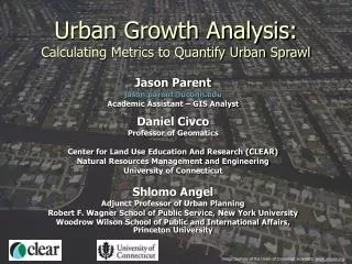
Urban Growth Analysis: Calculating Metrics to Quantify Urban Sprawl. Jason Parent jason.parent@uconn.edu Academic Assistant – GIS Analyst Daniel Civco Professor of Geomatics Center for Land Use Education And Research (CLEAR) Natural Resources Management and Engineering

E N D
Urban Growth Analysis:Calculating Metrics to Quantify Urban Sprawl Jason Parent jason.parent@uconn.edu Academic Assistant – GIS Analyst Daniel Civco Professor of Geomatics Center for Land Use Education And Research (CLEAR) Natural Resources Management and Engineering University of Connecticut Shlomo Angel Adjunct Professor of Urban Planning Robert F. Wagner School of Public Service, New York University Woodrow Wilson School of Public and International Affairs, Princeton University Image courtesy of the Union of Concerned Scientists: www.ucsusa.org
Project Overview • Analyze change in urban spatial structure, over a 10 year period, for a global sample of 120 cities. • Phase I (Angel et al. 2005): Acquire and / or derive necessary data. Develop preliminary set of metrics • Phase II (Angel et al. 2007): Further develop metrics to quantify and characterize the spatial structure of the cities. Create maps to facilitate qualitative assessment of the urban structure
CategoryGrid cell value 0 No Data 1 Other 2 Water 3 Urban Phase I: Land Cover Derivation • Land cover derived from Landsat satellite imagery. • Land cover derived for two dates: T1 (circa 1990) and T2 (circa 2000). • Land cover contained 3 categories: urban, water, and other
Phase I: Acquisition of City Boundaries • Administrative districts (i.e. Census tracts) acquired for each city. • Population data were attributed to the administrative districts. • Interpolated population values at land cover dates. • Districts define the outer perimeter of the cities and provide population data.
Phase I: Slope • Slope grid derived from Shuttle Radar Topography Mission Digital Elevation Models. • Slope calculated in percent. • Maximum slope defined as the slope value below which 99% of the urban area exists.
Phase II: The Metrics • Several sets of metrics were developed to measure specific aspects of the urban spatial structure • A total of 65 metrics have been developed • This presentation presents a sample of metrics from each set • Angel et. al. (2007) • The complete set of metrics will be presented in future papers at the conclusion of the study
Sprawl manifestations exhibited by the built-up area: Multiple urban cores Ribbon or strip developments Scatter developments Fragmented and unusable open space Manifestations are quantified with the following metrics: Main core Secondary core(s) Urban fringe Ribbon development Scatter development Sprawl Manifestations
Manifestation metrics based on the “urbanness” of the neighboring area Urbanness = % of pixels in neighborhood that are built-up The neighborhood is a 1 km2 circle centered on each pixel Sprawl Manifestation MetricsDerivation 252 pixels = 0.2 km2 Urbanness = 0.2 / 1 = 20%
Sprawl Manifestation MetricsDefinitions Built-up 30 to 50% urban < 30% urban > 50% urban Linear semi-contiguous groups approx. 100 meters wide Largest contiguous group of pixels All other groups All other groups Secondary core Main core Fringe Ribbon Scatter
Attributes of Urban Sprawl • Sprawl attributes are quantifiable for each city • A set of metrics was developed to describe each attribute • Metrics in each set tend to be correlated • Five attributes of urban spatial structure commonly associated with ‘sprawl’…
The First Attribute: the extension of the area of cities beyond the walkable range and the emergence of ‘endless’ cities: Landsat image Built-up area (impervious surfaces) Open space (OS) Urbanized OS (> 50 % built-up) Peripheral OS (< 100 m from built-up) Urbanized area Urban footprint
The Second Attribute: the persistent decline in urban densities and the increasing consumption of land resources by urban dwellers • Population densities based on the 3 types of urban extent: • Built-up area density • Urbanized area density • Urban footprint density
Minimum Average Distance (MAD) center The point that has the minimum distance to all other points in the urbanized area Central Business District (CBD) The point defining the original city center Determined by field surveys The Third Attribute: ongoing suburbanization and the decreasing share of the population living and working in metropolitan centers • City center shift: the distance between the MAD center and the CBD
Decentralization: Based on average distance to the MAD center for the urbanized area Normalized by the average distance to center of a circle with an area equal to the urbanized area Distance to center The Third Attribute: ongoing suburbanization and the decreasing share of the population living and working in metropolitan centers
Cohesion: Based on average interpoint distance of urbanized area Normalized by average interpoint distance of a circle with an area equal to the urbanized area Interpoint Distance The Third Attribute: ongoing suburbanization and the decreasing share of the population living and working in metropolitan centers
The Fourth Attribute: the diminished contiguity of the built-up areas of cities and the increased fragmentation of open space in and around them • Openness index: the average percent of open space within a circular 1 km2 neighborhood for all built-up pixels. • Open space contiguity: the probability that a built-up pixel will be adjacent to an open space pixel. • Open space fragmentation: the ratio of the combined urbanized and peripheral open space area to the built-up area.
The Fourth Attribute ContinuedNew Development • Development occurring between time periods T1 and T2 • Classification based on location relative to the T1 urban area • Infill: new development occurring within the T1 urbanized open space • Extension: new non-infill development intersecting the T1 urban footprint • Leapfrog: new development not intersecting the T1 urban footprint
The Fifth Attribute: the increased compactness of cities as the areas between their fingerlike extensions are filled in. • These metrics take the circle to be the shape of maximum compactness • Sprawl circle: the circle with the same average distance to center as the average distance to center of the urbanized area. • Radius = 1.5 * distance to center
area of the urbanized area (km2) buildable area of the sprawl circle (km2) Bacolod The Fifth AttributeMetrics • Single point compactness: area of the urbanized area (km2) SPC = area of the sprawl circle (km2) • Constrained single point compactness: CSPC =
The Urban Growth Analysis Tool (UGAT) • Python script that works with ArcGIS 9.2 • Executable through python or ArcGIS toolbox • UGAT performs all analyses needed to derive the metrics and create GIS layers • Data are input into the tool via a table • Table may contain data for any number of cities • UGAT will run the analysis for each city listed in the table
Conclusions • Phase II is currently ongoing as is development of the Urban Growth Analysis Tool. Future papers will provide in-depth and comprehensive discussions of the metrics developed in this project • The metrics, developed so far in this project, allow rigorous quantitative assessment of the change in urban spatial structure over time • Metrics in a set tend to be highly correlated • provides alternative ways to measure each attribute. • some metrics may be more practical than others • The Urban Growth Analysis Tool will facilitate the application of this analysis to other cities
References • Angel, S, J. R. Parent, and D. L. Civco. May 2007. Urban Sprawl Metrics: An Analysis of Global Urban Expansion Using GIS. ASPRS May 2007 Annual Conference. Tampa, FL • Angel, S, S. C. Sheppard, D. L. Civco, R. Buckley, A. Chabaeva, L. Gitlin, A. Kraley, J. Parent, M. Perlin. 2005. The Dynamics of Global Urban Expansion. Transport and Urban Development Department. The World Bank. Washington D.C., September.
QUESTIONS? Urban Growth Analysis:Calculating Metrics to Quantify Urban Sprawl Jason Parent jason.parent@uconn.edu Academic Assistant – GIS Analyst Daniel Civco Professor of Geomatics Center for Land Use Education And Research (CLEAR) Natural Resources Management and Engineering University of Connecticut Shlomo Angel Adjunct Professor of Urban Planning Robert F. Wagner School of Public Service, New York University Woodrow Wilson School of Public and International Affairs, Princeton University Image courtesy of the Union of Concerned Scientists: www.ucsusa.org