Download
1 / 10
110 likes | 363 Views
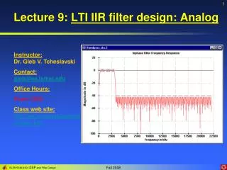
Lecture 9: LTI IIR filter design: Analog. Instructor: Dr. Gleb V. Tcheslavski Contact: gleb@ee.lamar.edu Office Hours: Room 2030 Class web site: http://ee.lamar.edu/gleb/dsp/index.htm. Considerations. First of all, design = determination of filter coefficients!.

E N D
Lecture 9: LTI IIR filter design: Analog Instructor: Dr. Gleb V. Tcheslavski Contact:gleb@ee.lamar.edu Office Hours: Room 2030 Class web site:http://ee.lamar.edu/gleb/dsp/index.htm
Considerations First of all, design = determination of filter coefficients! We are interested in BIBO systems! Usually, frequency response (its magnitude) is given by the specifications. Our goal is to find the filter coefficients while satisfying specs. Additional requirements on phase distortions (i.e. group delay and, therefore, phase characteristic) may give other constrains. Two ways to design a digital filter 1. Directly digital 2. From analog filters
Specs… Peak passband ripple: (9.3.1) Minimum stopband attenuation: (9.3.2) Maximum passband attenuation: (9.3.3)
Butterworth LPF (9.4.1) Here, N is an order of the filter; and c – cutoff frequency – corresponds to the -3 dB point. First 2N - 1 derivatives of (9.4.1) are zero at = 0. As a result, a Butterworth LPF is said to have maximally flat magnitude at = 0. This filter is completely determined by its order N and the cutoff frequency. The gain: (9.4.2) The gain at DC is 0 dB and at the cutoff frequency is at -3 dB. (9.4.1) decreases monotonically with frequency.
Butterworth LPF (9.5.1) (9.5.2) Analog poles: (9.5.3) (9.5.4) Poles of (9.5.1) occur on a circle of radius c at equally spaced points. An all pole filter.
Butterworth LPF (9.6.1) (9.6.2) (9.6.3) (9.6.4) (9.6.5) (9.6.6) We can solve both (9.6.6) and (9.6.7) for c and then use the average value. (9.6.7)
Chebyshev LPF There are two types of Chebyshev filter: Type I: equiripple in PB monotonic in SB Type II: equiripple in SB monotonic in PB (9.7.2) (9.7.1) Here, the Chebyshev polynomial: (9.7.3)
Chebyshev LPF The Chebyshev polynomials can also be generated by recursion: (9.8.1) where T0(x) = 1 and T1(x) = x. The order: (9.8.2) Type I – all pole Type II – zero-pole Poles on the ellipse
Elliptic (Cauer) LPF (9.9.1) Here UNis the Jacobian elliptic function (tabulated). This filter is equiripple in PB and SB – zero-pole filter. For the given order, elliptic filter has “the fastest transition” from PB to SB. Explicit expression for the filter order includes evaluation of elliptic integral, therefore, the order is usually determined experimentally. Elliptic filter is optimal in terms of approximation error but its phase response is worse than for B. and C.
Bessel LPF (9.10.1) Nth order Bessel polynomial: (9.10.2) where: (9.10.3) Alternatively: (9.10.4) Very ill defined in PB Linear phase in PB – to be destroyed later


![[f´‚nE˘RIks]](https://cdn0.slideserve.com/1072532/f-ne-riks-dt.jpg)