Edges and Binary Images
This text delves into the fundamentals of edge detection in image processing, elaborating on various filtering techniques, including median and Gaussian filters. It discusses the importance of identifying edges through gradient analysis and the mathematical principles behind convolution and differentiation. Key methods like the Canny edge detector are examined, highlighting their steps such as smoothing, thresholding, and non-maximum suppression. Additional insights on the impact of noise and the selection of scale parameters for Gaussian kernels are also addressed, providing a comprehensive overview for practitioners in the field.

Edges and Binary Images
E N D
Presentation Transcript
Edges and Binary Images Dan Witzner Hansen
What filter is likely to have produced this image output? filtered output original
Is the meadian filter a linear filter (convolution)? 5 x 5 median filter 25 x 25 median filter 50 x 50 median filter
Edge detection • Goal: map image from 2d array of pixels to a set of curves or line segments or contours. • Why? • Main idea: look for strong gradients, post-process Figure from J. Shotton et al., PAMI 2007
What can cause an edge? Depth discontinuity: object boundary Reflectance change: appearance information, texture Cast shadows Change in surface orientation: shape
intensity function(along horizontal scanline) first derivative edges correspond toextrema of derivative Derivatives and edges An edge is a place of rapid change in the image intensity function. image Source: L. Lazebnik
Recall : Images as functions Edges look like steep cliffs Source: S. Seitz
Differentiation and convolution For 2D function, f(x,y), the partial derivative is: For discrete data, we can approximate using finite differences: To implement above as convolution, what would be the associated filter?
Partial derivatives of an image -1 1 1 -1 ? -1 1 or Which shows changes with respect to x? (showing flipped filters)
Assorted finite difference filters >> My = fspecial(‘sobel’); >> outim = imfilter(double(im), My); >> imagesc(outim); >> colormap gray;
Image gradient The gradient of an image: The gradient points in the direction of most rapid change in intensity The gradient direction (orientation of edge normal) is given by: The edge strength is given by the gradient magnitude Slide credit S. Seitz
Effects of noise Consider a single row or column of the image Plotting intensity as a function of position gives a signal Where is the edge?
Solution: smooth first Look for peaks in Where is the edge?
Derivative theorem of convolution Differentiation property of convolution.
0.0030 0.0133 0.0219 0.0133 0.0030 0.0133 0.0596 0.0983 0.0596 0.0133 0.0219 0.0983 0.1621 0.0983 0.0219 0.0133 0.0596 0.0983 0.0596 0.0133 0.0030 0.0133 0.0219 0.0133 0.0030 Derivative of Gaussian filter Why is this preferable?
Derivative of Gaussian filters y-direction x-direction Source: L. Lazebnik
Laplacian of Gaussian Consider Laplacian of Gaussian operator Where is the edge? Zero-crossings of bottom graph
2D edge detection filters Laplacian of Gaussian Gaussian derivative of Gaussian • is the Laplacianoperator (trace of Hessian):
Mask properties • Smoothing • Values positive • Sum to 1 constant regions same as input • Amount of smoothing proportional to mask size • Remove “high-frequency” components; “low-pass” filter • Derivatives • Opposite signs used to get high response in regions of high contrast • Sum to 0 no response in constant regions • High absolute value at points of high contrast • Filters act as templates • Highest response for regions that “look the most like the filter” • Dot product as correlation
Gradients -> edges Primary edge detection steps: 1. Smoothing: suppress noise 2. Edge enhancement: filter for contrast 3. Edge localization Determine which local maxima from filter output are actually edges vs. noise • Threshold, Thin ( more about this later)
Smoothing with a Gaussian Recall: parameter σ is the “scale” / “width” / “spread” of the Gaussian kernel, and controls the amount of smoothing. …
Effect of on derivatives σ = 1 pixel σ = 3 pixels The apparent structures differ depending on Gaussian’s scale parameter. Larger values: larger scale edges detected Smaller values: finer features detected
So, what scale to choose? Too fine of a scale…can’t see the forest for the trees. Too coarse of a scale…can’t tell the maple grain from the cherry.
Canny edge detector • Filter image with derivative of Gaussian • Find magnitude and orientation of gradient • Non-maximum suppression: • Thin multi-pixel wide “ridges” down to single pixel width • Linking and thresholding (hysteresis): • Define two thresholds: low and high • Use the high threshold to start edge curves and the low threshold to continue them • MATLAB: edge(image, ‘canny’); • >>help edge Source: D. Lowe, L. Fei-Fei
The Canny edge detector original image (Lena)
The Canny edge detector norm of the gradient
The Canny edge detector thresholding
The Canny edge detector How to turn these thick regions of the gradient into curves? thresholding
Non-maximum suppression Check if pixel is local maximum along gradient direction, select single max across width of the edge requires checking interpolated pixels p and r
The Canny edge detector Problem: pixels along this edge didn’t survive the thresholding thinning (non-maximum suppression)
Hysteresis thresholding • Check that maximum gradient value is sufficiently large • drop-outs? use hysteresis • use a high threshold to start edge curves and a low threshold to continue them. Source: S. Seitz
high threshold (strong edges) low threshold (weak edges) hysteresis threshold Hysteresis thresholding original image Source: L. Fei-Fei
Object boundaries vs. edges Shadows Background Texture
Seam Carving uses edges to be able to resize images • Try it.
Thresholding • What is thresholding? • Choose a threshold value t • Set any pixels less than t to zero (off) • Set any pixels greater than or equal to t to one (on)
Binary images • Two pixel values • Foreground and background • Mark region(s) of interest
Thresholding • Given a grayscale image or an intermediate matrix threshold to create a binary output. Example: edge detection Gradient magnitude fg_pix = find(gradient_mag > t); Looking for pixels where gradient is strong.
Thresholding • Given a grayscale image or an intermediate matrix threshold to create a binary output. Example: background subtraction - = Looking for pixels that differ significantly from the “empty” background. fg_pix = find(diff > t);
Thresholding • Given a grayscale image or an intermediate matrix threshold to create a binary output. Example: intensity-based detection fg_pix = find(im < 65); Looking for dark pixels
Thresholding • Given a grayscale image or an intermediate matrix threshold to create a binary output. Example: color-based detection fg_pix = find(hue > t1 & hue < t2); Looking for pixels within a certain hue range.
Issues • How to indentify multiple regions of interest? • Count objects • Compute further features per object • What to do with “noisy” binary outputs? • Holes • Extra small fragments
Issues • How to demarcate multiple regions of interest? • Count objects • Compute further features per object • What to do with “noisy” binary outputs? • Holes • Extra small fragments
Morphological operators • Change the shape of the foreground regions/ objects. • Useful to clean up result from thresholding • Basic operators are: • Dilation • Erosion • Combine • Opening • Closing
Dilation • Expands connected components • Grow features • Fill holes After dilation Before dilation