Download
1 / 18
190 likes | 323 Views
II. General equilibrium approaches—theory. A. Analytical tools. Producer’s problem Consumer’s problem Aggregate income and expenditure Markets and trade Distortions and non-traded goods. Producer’s problem. Consumer’s problem. Aggregate budget constraint. Equilibrium: Walras’ law.

E N D
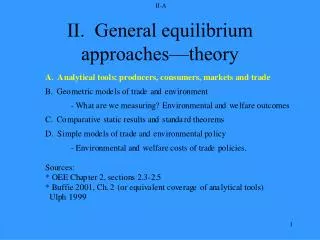
II-A II. General equilibrium approaches—theory
II-A A. Analytical tools • Producer’s problem • Consumer’s problem • Aggregate income and expenditure • Markets and trade • Distortions and non-traded goods
II-A Producer’s problem
II-A Consumer’s problem
II-A Aggregate budget constraint
II-A Equilibrium: Walras’ law
II-A Equilibrium of a two-sector economy y2 p = p2/p1 y = (y1, y2) m2 c = (c1, c2) u y1 m1
II-A Trade policy distortions • E.g. trade policy. • Define tariff-distorted prices p* = p(1 + t). • TEF is now: • e(p*, u) = r(p*, v) + t•m
II-A Externalities • E.g. env. externality in production • TEF is now: • e(p, u) = r(p, v) - z'y • where z is qty of pollution per unit of y produced. • Env. externality in consumption: u = u(c, z) ==> e(p, z, u) • NB assumption of separability.
II-A Non-traded goods • Goods may be non-traded (or effectively so) for intrinsic and policy reasons. • If one good is non-traded, for this, mn = 0. • Equilibrium now requires additional equation: • e(p, u) = r(p, v) • en(p, u) = rn(p, v) • and solves for pn as well as agg. welfare. • With endog. prices, preferences play a role.
II-A Salter-Swann diagram T RER = pN/pT (yT, yN) = (cT, cN) N
II-A Effects of growth T N
II-A Equilibrium: macro view (A) Base model Y = C + I + G + (X - M) let C + I + G = E be agg. dom. spending; so Y - E = X - M in equilibrium. Internal balance <==> external balance (B) With taxes and int’l capital flows Y + R - T = C + I + G - T + (X + R - M) let Y + R - T - C = S be agg. dom. savings; so X + R - M = (S - I) + (T - G) in eq’m. Curr. acc. surplus is equal to excess of savings over investment plus gov’t budget surplus.
II-A Summary • Basic tools reflect our assumptions about technology, preferences and behavior • Representative agent models • Focus of trade as determinant of price formation • Aggregate budget constraints impose internal consistency • Many forms of complication are possible.
II-A Q & A: basic tools