Download
1 / 104
1.05k likes | 1.71k Views
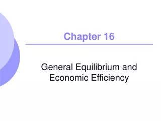
Chapter 16. General Equilibrium and Economic Efficiency. Topics to be Discussed. General Equilibrium Analysis Efficiency in Exchange Equity and Efficiency Efficiency in Production. Topics to be Discussed. The Gains from Free Trade On Overview--The Efficiency of Competitive Markets

E N D
Chapter 16 General Equilibrium and Economic Efficiency
Topics to be Discussed • General Equilibrium Analysis • Efficiency in Exchange • Equity and Efficiency • Efficiency in Production Chapter 16
Topics to be Discussed • The Gains from Free Trade • On Overview--The Efficiency of Competitive Markets • Why Markets Fail Chapter 16
General Equilibrium Analysis • Up to this point, we have been focused on partial equilibrium analysis • Activity in one market is has little or no effect on other markets. • Market interrelationships can be important • Complements and substitutes • Increase in firms input demand can cause market price of the input and product to rise Chapter 16
General Equilibrium Analysis • To study how markets interrelate, we can use general equilibrium analysis • Simultaneous determination of the prices and quantities in all relevant markets, taking into account feedback effects. • The feedback effect is the price or quantity adjustment in one market caused by price and quantity adjustments in related markets Chapter 16
Two Interdependent Markets – Moving to General Equilibrium • Scenario • The competitive markets of: • DVD rentals • Movie theater tickets • These goods are substitutes • Changing prices in one market are likely to affect the other market Chapter 16
Two Interdependent Markets – Moving to General Equilibrium • Scenario • Equilibrium price of movies is $6.00 • Equilibrium price of DVD rentals are $3.00 • Government places a $1.00 tax on each movie ticket • Need to look at effect of tax on • Market for DVDs • Feedback effects in Movie market Chapter 16
S*M SM SV $3.50 $6.35 $3.00 D’V $6.00 DM DV QV Q’V Q’M QM Two Interdependent Markets – Movies and DVDs $1 tax on each movie ticket causes supply to fall General Equilibrium Analysis: Increase in movie ticket prices increases demand for videos. Price Price Number of Movie Tickets Number of Videos
$6.82 S*M SM SV $3.58 $6.75 $3.50 $6.35 D*M D*V $3.00 D’V $6.00 D’M DM DV Q*M Q*V Number of Movie Tickets Q”M QV Q’V Q’M QM Two Interdependent Markets – Movies and DVDs The increase in the price of videos increases the demand for movies. General Equilibrium Analysis: The Feedback effects continue. Price Price Number of Videos Chapter 16
Two Interdependent Markets – Movies and DVDs • Observation • Without considering the feedback effect with general equilibrium, the impact of the tax would have been underestimated • This is an important consideration for policy makers. • You can check for yourself that in the market for complements, the tax would be overestimated Chapter 16
Reaching General Equilibrium • Must be able to determine the equilibrium price of both movies and DVDs simultaneously • We must simultaneously find two prices that equate quantity demanded and quantity supplied in all related markets • The requires finding the solution to four equations: demand and supply for DVDs and Movies Chapter 16
The Interdependence of International Markets • Brazil and the United States compete in the world soybean market so one market can affect the other. • Brazil limited exports of soybeans in the late 1960’s and early 1970’s causing price in Brazil to fall. • Eventually the export controls were to be removed, and Brazilian exports were expected to increase. Chapter 16
The Interdependence of International Markets • Expectation was based on partial equilibrium analysis • Program actually increased the price and production of soybeans in US as well as US exports • This caused brazil to have difficulties exporting even after control was removed • Can show how each market was effected and compare to general equilibrium analysis Chapter 16
Efficiency in Exchange • We showed before that competitive markets are efficient because consumer and producer surplus are maximized • We can study this in more detail by examining an exchange economy • Market in which two or more consumers trade two goods among themselves • Same for two countries Chapter 16
Efficiency in Exchange • An efficient allocation of goods is one where no one can be made better off without making someone else worse off • Pareto efficiency • Voluntary trade between two parties is mutually beneficial and increases economic efficiency. Chapter 16
The Advantages of Trade • Assumptions • Two consumers (countries) • Two goods • Both people know each others preferences • Exchanging goods involves zero transaction costs • James & Karen have a total of 10 units of food and 6 units of clothing. Chapter 16
The Advantage of Trade • To determine if they are better off, we need to know the preferences for food and clothing Chapter 16
The Advantage of Trade • Karen has a lot of clothing and little food. • MRS of food for clothing is 3 • To get 1 unit of food, she will give up 3 units of clothing • James’ MRS of food for clothing is only ½ • He will give up ½ unit if clothing for 1 unit of food Chapter 16
The Advantage of Trade • There is room for trade • James values clothing more than Karen • Karen values food more than James • Karen willing to give up 3 units of clothing to get 1 unit of food, but James is willing to take only ½ unit of clothing for 1 unit of food • Actual terms of trade are determined through bargaining • Trade for 1 unit of food will fall between ½ and 3 units of clothing Chapter 16
The Advantage of Trade • Suppose Karen offers James 1 unit of clothing for 1 unit of food • James will have more clothing, which he values food • Karen will have more food, which she values more • Whenever two consumers’ MRSs are different, there is room for mutually beneficial trade • Allocation of resources is inefficient Chapter 16
The Advantage of Trade • From this analysis we obtain an important result: An allocation of goods is efficient only if the goods are distributed so that the marginal rate of substitution between any pair of goods is the same for all consumers. Chapter 16
The Edgeworth Box Diagram • A diagram showing all possible allocations of either two goods between two people or of two inputs between two production processes is called an Edgeworth Box Chapter 16
The Edgeworth Box Diagram • Food is measured across the horizontal axis • Clothing is measured on the vertical axis • Length of box is the total amount of food – 10 units • Height of box is the total amount of clothing – 6 units Chapter 16
The Edgeworth Box Diagram • Each point describes the market baskets of both consumers • James’ basket is read from origin OJ • Karen’s basket is read from origin OK, in the reverse direction • James has 7 units of food and 1 unit of clothing – point A • Karen has 3 units of food and 5 units of clothing – point A from different axis Chapter 16
Karen’s Food 3F James’s Clothing Karen’s Clothing 5C 1C A 7F James’s Food Exchange in an Edgeworth Box 10F 0K 6C The initial allocation before trade is A: James has 7F and 1C & Karen has 3F and 5C. 6C 0J 10F
Karen’s Food 10F 4F 3F 0K 6C James’s Clothing Karen’s Clothing B 2C 4C 5C 1C A 6C 0J 6F 7F 10F James’s Food Exchange in an Edgeworth Box The allocation after trade is B: James has 6F and 2C & Karen has 4F and 4C. +1C -1F Chapter 16
Efficient Allocations • A trade from A to B makes both Karen and James better off • Is it efficient? • If James’s and Karen’s MRS are the same at B the allocation is efficient. • This depends on the shape of their indifference curves. Chapter 16
Efficient Allocations • James’ indifference curves are drawn as we usually see them • Karen’s indifference curves are rotated 180o convex to her axis • The indifference curves that go through point A have different slopes and therefore different MRSs • The allocation is not efficient Chapter 16
Efficient Allocations • The shaded area between these two indifference curves represents all the possible allocations of food and clothing that would make both James and Karen better off than A • Describes all mutually beneficial trades Chapter 16
Efficient Allocations • We can see both parties are better off at point B since they both end up on a higher indifference curve • Not efficient since MRSs different – indifference curve have different slopes • Although a trade might make both parties better off, the new allocation is not necessarily efficient Chapter 16
Efficient Allocations • How do these parties reach an efficient allocation? • When there is no more room for trade • When their MRSs are equal • They will keep trading, reaching higher indifference curves, until they can no longer do so and still make each better off • This is when indifference curves are tangent – they have the same slope and same MRS Chapter 16
Karen’s Food James’s Clothing Karen’s Clothing A Gains from trade UJ1 UK1 James’s Food Efficiency in Exchange 10F 0K 6C A: UJ1 = UK1, but the MRS is not equal. All combinations in the shaded area are preferred to A. 6C 0J 10F Chapter 16
Karen’s Food D UJ3 C UK2 James’s Clothing Karen’s Clothing B UJ2 UK3 A UJ1 UK1 James’s Food Efficiency in Exchange 10F 0K 6C D is also a possible efficient allocation depending on bargaining At point C, MRSs are equal and allocation is efficient Point B is on higher IC but is not efficient 6C 0J 10F Chapter 16
Any move outside the shaded area will make one person worse off (closer to their origin). B is a mutually beneficial trade--higher indifference curve for each person. Trade may be beneficial but not efficient. MRS is equal when indifference curves are tangent and the allocation is efficient. 10F Karen’s Food 0K 6C D Karen’s Clothing James’s Clothing C UJ3 B UJ2 A UJ1 6C UK3 UK2 UK1 0J 10F James’s Food Efficiency in Exchange Chapter 16
Efficiency in Exchange • The Contract Curve • To find all possible efficient allocations of food and clothing between Karen and James, we would look for all points of tangency between each of their indifference curves. • The contract curve shows all the efficient allocations of goods between two consumers, or of two inputs between two production functions Chapter 16
Contract Curve G F E The Contract Curve Karen’s Food 0K E, F, & G are Pareto efficient . James’s Clothing Karen’s Clothing 0J Chapter 16 James’s Food
Contract curve • All points of tangency between the indifference curves are efficient. • MRS of individuals is the same • No more room for trade • The contract curve shows all allocations that are Pareto efficient. • Pareto efficient allocation occurs when further trade will make someone worse off. Chapter 16
Efficiency in Exchange • Application: The policy implication of Pareto efficiency when removing import quotas: • Remove quotas • US Consumers gain • Some US workers lose • Removal of quotas and subsidies to the workers Chapter 16
Efficiency in Exchange • US consumers would be better off and after a time, the US workers are no worse off and might be better off • Package will increase efficiency • Efficiency therefore can be reached with the combined set of changes leaves someone better off and no one worse off Chapter 16
Efficiency in Exchange • Consumer Equilibrium in a Competitive Market • Competitive markets have many actual or potential buyers and sellers, so if people do not like the terms of an exchange, they can look for another seller who offers better terms. Chapter 16
Consumer Equilibrium in a Competitive Market • There are many Jameses and Karens. • They are price takers • Relative price of food and clothing = 1 • Trade depends on relative prices, not actual prices Chapter 16
Consumer Equilibrium in a Competitive Market • We can show opportunities for trade for many consumers • When prices of food and clothing are equal, we can show the price line, PP’ with a slope of –1 • Shows all possible allocations that exchange can achieve • James buys 2 clothing for 2 food: A to C • Karen buys 2 food for 2 clothing: A to C • Both increase satisfaction Chapter 16
Price Line P C UJ2 A UJ1 P’ UK2 UK1 Consumer Equilibrium in a Competitive Market 10F 0K Karen’s Food 6C Begin at A: Each James buys 2C and sells 2F moving from Uj1 to Uj2, which is preferred (A to C). Begin at A: Each Karen buys 2F and sells 2C moving from UK1 to UK2, which is preferred (A to C). Karen’s Clothing James’s Clothing 6C 0J 10F James’s Food Chapter 16
Consumer Equilibrium in a Competitive Market • The amount of clothing that Karen wanted to sell is equal to the amount of clothing that James wanted to buy • An equilibrium is a set of prices at which the quantity demanded equals the quantity supplied in every market • Also called competitive equilibrium Chapter 16
Consumer Equilibrium in a Competitive Market • Not all prices lead to equilibrium • If the MRSs of the players is not equal, then we are not in equilibrium • If the price of food is 1 and price of clothing is 3 • James is unwilling to trade, MRS = ½ • Karen is happy to sell clothing at that price but has no one to sell to • Market is in disequilibrium Chapter 16
Consumer Equilibrium in a Competitive Market • Disequilibrium is only temporary in competitive market • Excess demand will cause price to rise • Excess supply will cause price to fall • In our example, we have excess supply of clothing and excess demand of food • Should expect the price of food to increase relative to price of clothing • Prices adjust until equilibrium is reached Chapter 16
Economic Efficiency of Competitive Markets • As shown before, we can see that the allocation in a competitive equilibrium is economically efficient • The efficient point must occur where the two indifference curves are tangent • If not, one of the consumers can increase their utility and be better off Chapter 16
Consumer Equilibrium in a Competitive Market • In a general equilibrium setting where all markets are perfectly competitive, we can show the same result • Best example of Adam Smith’s invisible hand • Economy will automatically allocate all resources efficiently without need for regulatory control • Supports argument for less government intervention and more highly competitive markets Chapter 16
Consumer Equilibrium in a Competitive Market • First Theorem of Welfare Economics • If everyone trades in a competitive market place, all mutually beneficial trades will be completed and the resulting equilibrium allocation of resources will be economically efficient • Welfare economics involves the normative evaluation of markets and economic policy Chapter 16