Download
1 / 60
600 likes | 734 Views
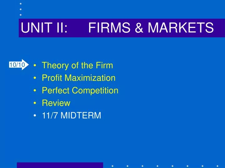
UNIT II: FIRMS & MARKETS. Theory of the Firm Profit Maximization Perfect Competition Review 11/7 MIDTERM. 10/10. Theory of the Firm.

E N D
UNIT II: FIRMS & MARKETS • Theory of the Firm • Profit Maximization • Perfect Competition • Review • 11/7 MIDTERM 10/10
Theory of the Firm Today we will build a model of the firm, based on the model of the consumer we developed in UNIT I. Where consumers attempt to maximize utility, firms attempt to maximize profit. We saw how changes in prices affect consumers’ optimal decisions and derived a demand function: P = f(Qd). Now we will see how changes in prices affect firms’ profit maximizing decisions and derive a supply curve: P = f(Qs). Later, we will put supply and demand together, and begin our analysis of markets and market structures.
Theory of the Firm The Good News! In moving from the consumer to the firm, we replace the troublesome notion of utilitywith something nice and hard-edged: profit. Where utility is subjective and thus hard to measure, now we’ll be talking about simple, measurable quantities, physical units of inputs (tons of steel, hours of labor) and outputs, and an account for everything in dollars and cents (“the bottom line”).
Theory of the Firm • The Technology of Production • Short-run v. Long-run • Isoquants • Returns to Scale • Cost Curves • Cost Minimization • Profit Maximization
Theory of the Firm First, we need to write down our model: Profit (P) = Total Revenue(TR) – Total Cost(TC) TR(Q) = PQ TC(Q) = rK + wL P Price L Labor Q Quantity K Capital w Wage Rate Q = f(K,L) r Rate on Capital The firm wants to maximize this difference
Theory of the Firm First, we need to write down our model: Profit (P) = Total Revenue(TR) – Total Cost(TC) TR = PQ TC(Q) = rK + wL P Price L Labor Q Quantity K Capital w Wage Rate Q = f(K,L) r Rate on Capital Economic costs include opportunity costs Economic P < Normal P (accounting) If a firm earns positive profits, all factors are earning more than they could in alternative uses
Theory of the Firm First, we need to write down our model: Profit (P) = Total Revenue(TR) – Total Cost(TC) TR(Q) = PQ TC(Q) = rK + wL P Price L Labor Q Quantity K Capital w Wage Rate Q = f(K,L) r Rate on Capital INPUTS The production functiondescribes a relationship between the quantity of physical inputs (K, L) and quantity of outputs (Q).
Theory of the Firm First, we need to write down our model: Profit (P) = Total Revenue(TR) – Total Cost(TC) TR(Q) = PQ TC(Q) = rK + wL P Price L Labor Q Quantity K Capital w Wage Rate Q = f(K,L) r Rate on Capital OUTPUT The production functiondescribes a relationship between the quantity of physical inputs (K, L) and quantity of output (Q).
The Technology of Production Technology: a list ofall possible production plans, i.e., all the ways to transform inputs into outputs. The production function: describes a relationship between inputs and the maximum quantity of output (all inputs are used technologically efficiently). Technological constraints: Nature (& science) imposes certain physical constraints on a firm: only so much output can be created out of so much input(s). Thus the firm must limit its choice to technologically feasible production plans.
The Technology of Production The Production Function Q = F(K, L), For a given technology Q Output L Labor K Capital Cobb-Douglas Production Function Q = AKaLb where A is a constant (scale).
Production in the Short-Run We define the short-run as the period in which at least one factor of production is fixed: Total Product Function The maximum quantity of output the can be produced for a given quantity of input, holding other factors constant. TP: Q = f(L) Q L
Production in the Short-Run We define the short-run as the period in which at least one factor of production is fixed: Law of Diminishing Marginal Returns As firm adds more of a variable factor (holding others constant), the increment to output will eventually decrease. Total Product Function TP: Q = f(L) Q L
Production in the Short-Run Average Product AP = Q/L Output per unit labor (input) A ray from the origin to any point on the TP curve is AP Q Q TP L AP L
Production in the Short-Run Average Product AP = Q/L Output per unit labor (input) AP is greatest at Point A Q Q A TP L AP L
Production in the Short-Run Marginal Product MPL=dQ/dL Increase in output from a unit increase in labor (input) The slope of TP curve is MP MP is greatest at point B Q Q A TP B L L MP
Production in the Short-Run Marginal Product MPL=dQ/dL Increase in output from a unit increase in labor (input) The slope of TP curve is MP MP is negative at point C Q Q C A TP B L L MP
Production in the Short-Run Marginal Product MPL=dQ/dL Increase in output from a unit increase in labor (input) The slope of TP curve is MP MP = AP at AP max Q Q C A TP B L AP L MP
Production in the Short-Run Average and Marginal Products In general, average will equal marginal, where average is greatest, e.g., the height of people in the room. Q Q C A TP B L AP L MP
Production in the Long-Run In the long run, all factors of production are variable. Total Product Function TP: Q = f(K,L) Q Again, we have 3 variables… K,L
Production in the Long-Run In the long run, all factors of production are variable. The production function determines the maximum possible output for a given combination of inputs (a boundary condition). Technological efficiency. Total Product Function TP: Q = f(K,L) Q K,L
Production in the Long-Run In the long run, all factors of production are variable. One particularly convenient form is theCobb-Douglas production function Q = AKaLb Total Product Function TP: Q = f(K,L) Q K,L
Production in the Long-Run In the long run, all factors of production are variable. Total Product Function TP: Q = f(K,L) Q K L
Production in the Long-Run Isoquant: all the possible combinations of inputs that are just sufficient to produce a given level of output. Well-behaved isoquants are monotonic and convex K Q = 20 Q = 10 L
Production in the Long-Run Isoquant: all the possible combinations of inputs that are just sufficient to produce a given level of output. Well-behaved isoquants are monotonic: More of any input produces at least as much output. MPL, MPK > 0. K Q = 20 Q = 10 L
Production in the Long-Run Isoquant: all the possible combinations of inputs that are just sufficient to produce a given level of output. Well-behaved isoquants are convex: Combinations of production plans produce at least as much as either alone. K aK bK 10 units of output can be produced using aL units of L and aK units of K or bL units of L and bK units of K or (aL+bL)/2 of L and (aK+bK)/2 of K or any linear combination of plans a and b Q = 20 Q = 10 aL bL L
Production in the Long-Run Isoquant: all the possible combinations of inputs that are just sufficient to produce a given level of output. Marginal Rate of Technical Substitution (MRTS): The rate at which one input can be exchanged for another while keeping output constant. K Q = 20 Q = 10 L
Production in the Long-Run Isoquant: all the possible combinations of inputs that are just sufficient to produce a given level of output. MRTSKL = - MPL/MPK Along an isoquant dQ = 0 dK*MPK +dL*MPL = 0 dK/dL = - MPL/MPK = slope K MRTS: The rate at which one input can be exchanged for another while keeping output constant. This is the slope of the isoquant. Q = 20 Q = 10 L
Returns to Scale Constant returns: doubling all inputs doubles output. The firm can replicate production unit (e.g., build another plant). K 2K K Q2 = 2Q1 Q = AKaLb a + b = 1 Q2 Q1 L 2L L
Returns to Scale Increasing returns: doubling all inputs more than doubles output. (aka “Economies of scale”). K 2K K Q2 > 2Q1 Q = AKaLb a + b > 1 Q2 Q1 L 2L L
Returns to Scale Decreasing returns: doubling all inputs less than doubles output. Crowding (assume homogeneous factor quality). K 2K K Q2 < 2Q1 Q = AKaLb a + b < 1 Q2 Q1 L 2L L
Returns to Scale Decreasing returns: doubling all inputs less than doubles output. Crowding (assume homogeneous factor quality). K 2K K Q2 < 2Q1 Firm should always be able to get at least constant returns by dividing production Q2 Q1 L 2L L
Returns to Scale Do any of these cases violate with the law of diminishing marginal productivity?
Cost Curves We can combinetechnological infoabout production possibilities withprice infoto characterize the firm’s cost structure. In the short-run, economic efficiency = technological efficiency, b/c to produce a certain level of output, Q, given K, there is a unique level of L required. This is the cheapest way to produce Q. In the long-run, all factors are variable, and the firm’s problem is to choose its optimal factor proportion.
Cost Curves We can combinetechnological infoabout production possibilities withprice infoto characterize the firm’scost structure. Q SR Total Product Function TP: Q = f(L) A firm will never choose to produce where MPL is negative. L
Cost Curves We can combinetechnological infoabout production possibilities withprice infoto characterize the firm’scost structure. SR Total Product Function TP: Q = f(L,K) SR Cost Function TVC = wL(Q) Q Qo $ wLo Lo L Qo Q
Cost Curves We can combinetechnological infoabout production possibilities withprice infoto characterize the firm’scost structure. SR Total Product Function TP: Q = f(L,K) SR Cost Functions TC = TFC + TVC TVC = wL(Q) TFC = rK Q Qo $ Lo L Qo Q The shape of cost curves come from technology
Cost Curves TC Average Cost AC = TC/Q Cost per unit output A ray from the origin to any point on the TC curve is AC AC min at point A $ $ A Q AC Q
Cost Curves TC Marginal Cost MC = dTC/dQ = dTVC/dQ (b/c only VC can change) = wdL/dQ = w/MPL MC min at point B $ $ B Q MC AC Q
Cost Curves TC Marginal Cost MC = dTC/dQ = dTVC/dQ (b/c only VC can change) = wdL/dQ = w/MPL AC = MC at ACmin $ $ A B Q MC AC Q
Cost Curves TC Average Fixed Cost AFC = TFC/Q Average Fixed Cost AVC = TVC/Q $ $ TVC A B TFC Q MC AC AVC AFC Q
Cost Curves 3 short-run total cost curves associated w/different levels of K. The cheapest way to produce Q1 is using SRTC1 … Deriving long-run cost curves: $ SRTC(K2) SRTC(K1) SRTC(K3) Q1 Q2 Q3 Q
Cost Curves 3 short-run total cost curves associated w/different levels of K. If K is continuously variable, the lower envelope of all SRTCs shows the lowest cost for each quantity of output. This is the long-run total cost curve Deriving long-run cost curves: $ LRTC Q1 Q2 Q3 Q
Cost Curves We can’t say much about the shape of the LRTC curve. (Shown is a cubic function, giving us s-shaped curves). Cobb-Douglas w/constant returns give us a linear (upward-sloping) curve. Deriving long-run cost curves: $ LRTC Q1 Q2 Q3 Q
Cost Curves 3 short-run average cost curves associated w/different levels of K. If K is continuously variable, the lower envelop of all SRACs is the long-run average cost curve. Deriving long-run cost curves: $ SRAC3 SRAC1 LRAC SRAC2 Q1 Q2 Q3 Q
Cost Curves 3 short-run marginal cost curves associated w/different levels of K. The long-run marginal cost curve is the locus of points along srmcs associated w/difference levels of output. Deriving long-run cost curves: $ SRMC2 SRMC3 LRMC SRMC1 Q1 Q2 Q3 Q
Cost Minimization Consider a firm that produces output according to the following production function. Q = 4K½L½ Assume that w = $18 and r = $36, and the firm currently has 16 units of capital. How much will it cost this firm to produce 10 units of output in the short-run?
Cost Minimization Consider a firm that produces output according to the following production function: Q = 4K½L½ Assume that w = $18 and r = $36, and the firm currently has 16 units of capital. With K = 16, the firm’s short-run production function is: Q = 16L½ For Q = 10, 10 = 16L½ => L = 100/256 = .39
Cost Minimization Consider a firm that produces output according to the following production function: Q = 4K½L½ Assume that w = $18 and r = $36, and the firm currently has 16 units of capital. To produce 10 units: 10 = 16L½ => L = 100/256 =.39 With K = 16, the firm’s total cost of production is: TC = rK + wL = 36(16) + 18(.39) = $583.03
Cost Minimization Consider a firm that produces output according to the following production function: Q = 4K½L½ Assume that w = $18 and r = $36, and the firm currently has 16 units of capital. More generally: Q = 16L½ => L = (Q/16)2 With K = 16, the firm’s short-run total cost function is: TC = rK + wL = 36(16) + 18(Q/16)2 = $576 + 18(Q/16)2
Cost Minimization in the Short-Run How much will it cost this firm to produce Q units of output in the short-run? Total Cost Function TCsr = 576 + 18(Q/16)2 $ Fixed Costs = rK = 36(16) = $576 Q