Download
1 / 27
320 likes | 522 Views
Explore the relationship between theoretical predictions and experimental measurements of vertical electric fields in the equatorial region, leading to the generation of intense plasma waves. Uncover the complexities of electron drift speeds, Doppler shifts, and differences in altitude-specific data. Understand the challenges of reconciling varying conductivities, neutral winds, and current densities across different coordinate systems.

E N D
E-Region Dynamo Theory and the DaytimeEquatorial Electrojet (second half part) Ya-Chih Mao April 2-3, 2019
Peak vertical electric fields in the range 10–20 mV/m have been predicted theoretically and would create electron drift speeds of 350–700 m/s. This exceeds the acoustic speed Cs, which is about 360 m/s, andleads to the generation of intense plasma waves via the two-stream instability. • Indeed, as we shall see,very large Doppler shifts occur when radar signals are scattered from the electrojet waves.
These observations show that the vertical electric field reaches values at least as large as that given by Ez= CsB9 mV/m at the very threshold of the two-stream instability, and it is very likely that the field reaches values half again as large.
The measurements in panels (a–c) have been combined in the right-hand panel to show the differential (net current) velocity as well as the E×B drift speed. At high altitudes the agreement is quite good, but below 104km there is a systematic difference. • As discussed in Chapter 2, neutral winds in the E region carry the ions with them but barely affect the electrons at all.
The systematic difference between the two curves in panel d suggests that a high, westward neutral wind may have been present, a result in agreement with TMA measurements made in the evening two days later (Larsen and Odom, 1997).
Notice that the measured current density in Fig. 3.17a field peaks almost 5km above the theoretical curve. This has been a mystery ever since Gagnepainet al. (1977). • A fix can be made by arbitrarily quadrupling the electron-ion collision frequency.
How do we derive the layer conductivities? • When do we consider the neutral wind? • When do we consider the vertical current? • How many coordinate systems and simplify conditions should be applied? • How does the conductivities vary in every degrees of freedom?
An electrojet theory suitable for comparison with such detailed data must include realistic altitude and latitude variations of σ. • Away from the equator, σ is often expressed in geographic rather than geomagnetic coordinates, and the resulting conductivity tensor is not as simple as (3.6). • If R is the rotation matrix relating geographic and geomagnetic coordinates, we have
where E’= E + U × B. Inserting the identity matrix I = R−1· R, we have • and we find a new tensor given by
For the simple case when geomagnetic and geographic north coincide and the dip angle is I, R corresponds to a rotation counterclockwise by the angle I about the x axis and
Application of σRto E’ determines J in the geographic coordinate system. • Following Forbes (1981), we denote the eastward direction as the λ axis, the northward as the θ axis, and the vertical as the z-axis. • Then
Note in this form that if we set I = 0, we recover a matrix identical to σ in (3.6). • Taking the divergence of J and substituting E = −∇φ, we have the dynamo equation
where the quantities are all measured in the earth-fixed frame and expressed in the rotated coordinate system. • This may be written as,
Even taking U and σRas known functions, this equation is a complicated partial differential equation with non-constant coefficients. • A common simplifying assumption is that no vertical current flows anywhere in the system; that is, all currents flow in a thin ionospheric shell. • Setting Jzequal to zero (in geographic coordinates now) yields
For I = 0 this reduces to (3.13) at the equator. • Using this expression to eliminate E‘z, JRcan now be written as a two-dimensional vector and the dynamo equation as a function of θ and λ only (Forbes, 1981), are the so-called layer conductivities.
Assuming E‘λand E‘θto be independent of height, (3.18) can be integrated over height to give the thin-shell dynamo equation
where the denote height-integrated layer conductivities, u and v are the zonal and meridional wind components, and Reis the radius of the earth. • It is important to note that assuming E’ = E + U × B to be independent of height implies that u, ν, and −∇φ are all independent of height, which is not very realistic.
Nonetheless, comparisons between the electrojet currents obtained using thin-shell theory and experimentally measured currents have been made by treating the zonal electric field as a free parameter (e.g., Sugiura and Cain, 1966; Untiedt, 1967) and by solving the dynamo equation by setting the zonal derivatives equal to zero.
However, the peak current density seems to be underestimated in these models, and details concerning the vertical and latitudinal extent of the electrojet are not reproduced. • More seriously, without vertical currents at the equator, which are suppressed by the thin-shell model, it is very hard to satisfy the divergence requirement since the electrojet varies rapidly in latitude but only slowly in longitude.
Forbes and Lindzen (1976) pointed out that allowing a vertical current could actually increase the electrojet intensity predicted by the models. • For example, returning to the current equation at the equator and again ignoring the neutral wind,
Eliminating Ezyields • Thus, if Jzis nonzero and positive at the equator, Jxwould exceed the Cowling current and the electrojet current would be stronger than σcEx.
The vertical electric field at the equator then becomes ( H/ P) Exrather than (σH/σP)Ex; that is, the integrated conductivities along the field line are used rather than the local values. • Above 100km the integrated conductivity ratio exceeds the local value so Jz0 and both the eastward current and the vertical electric field are greater than the thin-shell model.
Only Difference between theory and rockets measured.
The conductivity tensor Page 79
In a steady state in this slab model, no vertical current may flow, and the vertical Pedersen current must exactly cancel the Hall current. This implies that and hence that Page 93