Download
1 / 40
1.73k likes | 6.35k Views
Lecture 11. Quantum Mechanics. Hartree-Fock Self-Consistent-Field Theory. Outline of today’s lecture Postulates in quantum mechanics… Schr ö dinger equation… Simplify Schr ö dinger equation: Atomic units, Born-Oppenheimer approximation Solve Schr ö dinger equation with approximations:

E N D
Lecture 11. Quantum Mechanics. Hartree-Fock Self-Consistent-Field Theory • Outline of today’s lecture • Postulates in quantum mechanics… • Schrödinger equation… • Simplify Schrödinger equation: • Atomic units, Born-Oppenheimer approximation • Solve Schrödinger equation with approximations: • Variation principle, Slater determinant, Hartree approximation, • Hartree-Fock, Self-Consistent-Field, LCAO-MO, Basis set
References • Molecular Quantum Mechanics, Atkins & Friedman (4th ed. 2005), Ch. 1 & 8 • Essentials of Computational Chemistry. Theories and Models, C. J. Cramer, • (2nd Ed. Wiley, 2004) Chapter 4 • Molecular Modeling, A. R. Leach (2nd ed. Prentice Hall, 2001) Chapter 2 • Introduction to Computational Chemistry, F. Jensen (1999) Chapter 3 • A Brief Review of Elementary Quantum Chemistry • http://vergil.chemistry.gatech.edu/notes/quantrev/quantrev.html • Molecular Electronic Structure Lecture • http://www.chm.bris.ac.uk/pt/harvey/elstruct/introduction.html • Wikipedia (http://en.wikipedia.org): Search for Schrödinger equation, etc.
x rij li i θi Potential Energy Surface & Quantum Mechanics • How do we obtain the potential energy E? • MM: Evaluate analytic functions (FF) • QM: Solve Schrödinger equation 3N (or 3N-6 or 3N-5) Dimension PES for N-atom system Continuum Modeling Atomistic Modeling Geometry Quantum Modeling Charge Force Field For geometry optimization, evaluate E, E’ (& E’’) at the input structure X (x1,y1,z1,…,xi,yi,zi,…,xN,yN,zN) or {li,θi,i}. Length 1m 0.1 nm 1 nm 1cm
The Schrödinger Equation The ultimate goal of most quantum chemistry approach is the solution of the time-independent Schrödinger equation. ? (1-dim) Hamiltonian operator wavefunction (solving a partial differential equation)
Postulate #1 of Quantum Mechanics • The state of a quantum mechanical system is completely specified by the wavefunction or state function that depends on the coordinates of the particle(s) and on time. • The probability to find the particle in the volume element located at r at time t is given by . (Born interpretation) • The wavefunction must be single-valued, continuous, finite, and normalized (the probability of find it somewhere is 1). • = <|> Probability density
Born Interpretation of the Wavefunction: Probability Density
Probability Density: Examples B = 0 A = 0 A = B nodes
Postulate #2 of Quantum Mechanics • Once is known, all properties of the system can be obtained • by applying the corresponding operators to the wavefunction. • Observed inmeasurements are only the eigenvalues a which satisfy • the eigenvalue equation • eigenvalue • eigenfunction • (Operator)(function) = (constant number)(the same function) • (Operator corresponding to observable) = (value of observable) Schrödinger equation: Hamiltonian operator energy with (Hamiltonian operator) (e.g. with )
Physical Observables & Their Corresponding Operators with (Hamiltonian operator) (e.g. with )
the same function • constant • number Observables, Operators & Solving Eigenvalue Equations: an Example
The Uncertainty Principle When momentum is known precisely, the position cannot be predicted precisely, and vice versa. When the position is known precisely, Location becomes precise at the expense of uncertainty in the momentum
Postulate #3 of Quantum Mechanics • Although measurements must always yield an eigenvalue, • the state does not have to be an eigenstate. • An arbitrary state can be expanded in the complete set of • eigenvectors ( as where n . • We know that the measurement will yield one of the values ai, but • we don't know which one. However, • we do know the probability that eigenvalue ai will occur ( ). • For a system in a state described by a normalized wavefunction , • the average value of the observable corresponding to is given by • = <|A|>
Atomic Units (a.u.) • Simplifies the Schrödinger equation (drops all the constants) • (energy) 1 a.u. = 1 hartree = 27.211 eV = 627.51 kcal/mol, • (length) 1 a.u. = 1 bohr = 0.52918 Å, • (mass) 1 a.u. = electron rest mass, • (charge) 1 a.u. = elementary charge, etc. (before) (after)
Born-Oppenheimer Approximation • Simplifies further the Schrödinger equation (separation of variables) • Nuclei are much heavier and slower than electrons. • Electrons can be treated as moving in the field of fixed nuclei. • A full Schrödinger equation can be separated into two: • Motion of electron around the nucleus • Atom as a whole through the space • Focus on the electronic Schrödinger equation
Born-Oppenheimer Approximation (before) (electronic) (nuclear) E = (after)
= = Variational Principle • Nuclei positions/charges & number of electrons in the molecule • Set up the Hamiltonian operator • Solve the Schrödinger equation for wavefunction , but how? • Once is known, properties are obtained by applying operators • No exact solution of the Schrödinger eq for atoms/molecules (>H) • Any guessed trial is an upper bound to the true ground state E. • Minimize the functional E[] by searching through all acceptable • N-electron wavefunctions
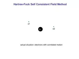
Hartree Approximation (1928)Single-Particle Approach Nobel lecture (Walter Kohn; 1998) Electronic structure of matter • Impossible to search through • all acceptable N-electron • wavefunctions. • Let’s define a suitable subset. • N-electron wavefunction • is approximated by • a product ofN one-electron • wavefunctions. (Hartree product)
Antisymmetry of Electrons and Pauli’s Exclusion Principle • Electrons are indistinguishable. Probability doesn’t change. • Electrons are fermion (spin ½). antisymmetric wavefunction • No two electrons can occupy the same state (space & spin).
= 0 Slater “determinants” • A determinant changes sign when two rows (or columns) are exchanged. • Exchanging two electrons leads to a change in sign of the wavefunction. • A determinant with two identical rows (or columns) is equal to zero. • No two electrons can occupy the same state. “Pauli’s exclusion principle” “antisymmetric” = 0
Hartree product is not antisymmetric! N-Electron Wavefunction: Slater Determinant • N-electron wavefunctionaprroximated by a product ofN one-electron • wavefunctions(hartree product). • It should be antisymmetrized ( ).
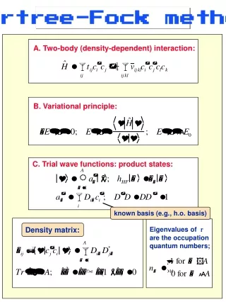
= ij Hartree-Fock (HF) Approximation • Restrict the search for the minimum E[] to a subset of , which • is all antisymmetric products of N spin orbitals (Slater determinant) • Use the variational principle to find the best Slater determinant • (which yields the lowest energy) by varying spin orbitals (orthonormal)
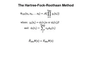
Slater determinant (spin orbital = spatial orbital * spin) Hartree-Fock (HF) Energy: Evaluation finite “basis set” Molecular Orbitals as linear combinations of Atomic Orbitals (LCAO-MO) where
where Hartree-Fock (HF) Equation: Evaluation • No-electron contribution (nucleus-nucleus repulsion: just a constant) • One-electron operator h (depends only on the coordinates of one electron) • Two-electron contribution (depends on the coordinates of two electrons)
Potential energy due to nuclear-nuclear Coulombic repulsion (VNN) *In some textbooks ESD doesn’t include VNN, which will be added later (Vtot = ESD + VNN). • Electronic kinetic energy (Te) • Potential energy due to nuclear-electronic Coulombic attraction (VNe)
Potential energy due to two-electron interactions (Vee) • Coulomb integral Jij (local) • Coulombic repulsion between electron 1 in orbital i and electron 2 in orbital j • Exchange integral Kij (non-local) only for electrons of like spins • No immediate classical interpretation; entirely due to antisymmetry of fermions > 0, i.e., a destabilization
Self-Interaction • Coulomb term J when i = j (Coulomb interaction with oneself) • Beautifully cancelled by exchange term K in HF scheme 0 = 0
and Hartree-Fock (HF) Equation • Fock operator: “effective” one-electron operator • two-electron repulsion operator (1/rij) replaced by one-electron operator VHF(i) • by taking it into account in “average” way Two-electron repulsion cannot be separated exactly into one-electron terms. By imposing the separability, the Molecular Orbital Approximation inevitably involves an incorrect treatment of the way in which the electrons interact with each other.
Self-Consistent Field (HF-SCF) Method • Fock operator depends on the solution. • HF is not a regular eigenvalue problem that can be solved in a closed form. • Start with a guessed set of orbitals; • Solve HF equation; • Use the resulting new set of orbitals • in the next iteration; and so on; • Until the input and output orbitals • differ by less than a preset threshold • (i.e. converged).
Koopman’s Theorem • As well as the total energy, one also obtains a set of orbital energies. • Remove an electron from occupied orbital a. Orbital energy = Approximate ionization energy
Electron Correlation • A single Slater determinant never corresponds to the exact wavefunction. • EHF > E0 (the exact ground state energy) • Correlation energy: a measure of error introduced through the HF scheme • EC = E0- EHF (< 0) • Dynamical correlation • Non-dynamical (static) correlation • Post-Hartree-Fock method • Møller-Plesset perturbation: MP2, MP4 • Configuration interaction: CISD, QCISD, CCSD, QCISD(T)