Quantum physics (quantum theory, quantum mechanics)

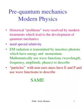
Quantum physics(quantum theory, quantum mechanics) Part 3

Summary of previous lecture • electron was identified as particle emitted in photoelectric effect • Einstein’s explanation of p.e. effect lends further credence to quantum idea • Geiger, Marsden, Rutherford experiment disproves Thomson’s atom model • Planetary model of Rutherford not stable by classical electrodynamics • Bohr atom model with de Broglie waves gives some qualitative understanding of atoms, but • only semiquantitative • no explanation for missing transition lines • angular momentum in ground state = 0 (1 ) • spin?? • Quantum mechanics: • Schrödinger equation describes observations • observables (position, momentum, angular momentum..) are operators which act on “state vectors” – wave functions

Homework from 2nd lecture • Calculate from classical considerations the force exerted on a perfectly reflecting mirror by a laser beam of power 1W striking the mirror perpendicular to its surface. • The solar irradiation density at the earth's distance from the sun amounts to 1.3 kW/m2 ; calculate the number of photons per m2 per second, assuming all photons to have the wavelength at the maximum of the spectrum , i.e.  ≈ max). Assume the surface temperature of the sun to be 5800K. • how close can an  particle with a kinetic energy of 6 MeV approach a gold nucleus? (q = 2e, qAu = 79e) (assume that the space inside the atom is empty space)

from The God Particle by Leon Lederman: Leaving his wife at home, Schrödinger booked a villa in the Swiss Alps for two weeks, taking with him his notebooks, two pearls, and an old Viennese girlfriend. Schrödinger's self-appointed mission was to save the patched-up, creaky quantum theory of the time. The Viennese physicist placed a pearl in each ear to screen out any distracting noises. Then he placed the girlfriend in bed for inspiration. Schrödinger had his work cut out for him. He had to create a new theory and keep the lady happy. Fortunately, he was up to the task. • Heisenberg is out for a drive when he's stopped by a traffic cop. The cop says, "Do you know how fast you were going?"Heisenberg says, "No, but I know where I am."

Compton scattering 1 • Scattering of X-rays on free electrons; • Electrons supplied by graphite target; • Outermost electrons in C loosely bound; binding energy << X ray energy •  electrons “quasi-free” • Expectation from classical electrodynamics: • radiation incident on free electrons  electrons oscillate at frequency of incident radiation  emit light of same frequency  light scattered in all directions • electrons don’t gain energy • no change in frequency of light

Compton (1923) measured intensity of scattered X-rays from solid target, as function of wavelength for different angles. Nobel prize 1927. X-ray source Collimator (selects angle) Crystal (selects wavelength)  Target Compton scattering 2 Result: peak in scattered radiation shifts to longer wavelength than source. Amount depends on θ(but not on the target material). A.H. Compton, Phys. Rev. 22 409 (1923)

θ Incident light wave Emitted light wave Oscillating electron Before After scattered photon Incoming photon Electron scattered electron Compton scattering 3 • Classical picture: oscillating electromagnetic field causes oscillations in positions of charged particles, which re-radiate in all directions at same frequency as incident radiation. No change in wavelength of scattered light is expected • Compton’s explanation: collisions between particles of light (X-ray photons) and electrons in the material

θ Before After scattered photon Incoming photon Electron scattered electron Compton scattering 4 Conservation of energy Conservation of momentum From this derive change in wavelength:

unshifted peaks come from collision between the X-ray photon and the nucleus of the atom ’ -  = (h/mNc)(1 - cos)  0 since mN >> me Compton scattering 5

Postulates of Quantum Mechanics • The state of a quantum mechanical system is completely specified by its wavefunction, (x,t) • For every classical observable there is a linear, Hermitian operator in quantum mechanics • In any measurement associated with an operator, the only values observed are eigenvalues of the operator, • The average value of an observable is given by its expectation value, • The wavefunction obeys the Schrödinger equation • H = “Hamiltonian” = energy operator =

measurement (1) • Measurement involves interaction with the system which is subject to the measurement process • Measurements always have “errors”, uncertainties, due to: • Imperfections of measuring equipment/process  uncertain data • System subject to random outside influences • Measurement result with quoted uncertainty is really a probabilistic statement: • really means • (assuming “gaussian errors”)

Measurement (2) • Any measurement disturbs the system  will be in a different state from the one it was in before the measurement • Examples: • Temperature measurement: thermometer gets into thermal equilibrium with measured system in- (or out-)flux of thermal energy temperature changed • Measure position of object – have to shine light onto it to see it, light photons transfer momentum to measured object • Influence of measurement process, as well as random outside influences (non-isolation) can more easily be minimized for big (high mass) system •  expect physics of small systems to be more probabilistic

Measurement (3) “Heisenberg microscope”: • Try to measure position of a tiny particle – image particle with a microscope\ • Uncertainty of particle position  angular resolution of microscope =1.22/D, where = wavelength of used light, D=diameter of objective lens • To optimize position resolution, need small wavelength and large D • p=h/, energetic photons need to be scattered off particle under large angles  momentum of particle changed • Requirement fro precise measurement of positionsignificant jolts to particle uncertainty of momentum

Measurement (4) • Scientific statement about a measurement is a prediction: • “momentum of this electron is 30.02 GeV/c” means: if you measure p, you will obtain (with 95% confidence) a value between 3-0.04 and 3+0.04 GeV/c • ideal measurement: • is reproducible • Subsequent measurement of the same quantity will yield the same result • brings the system into a special state that has the property of being unaffected by a further measurement of the same type

Measurement(5): Quantum states • Existence of quantum states is one of the postulates of QM • Any system has quantum states in which the outcome of a measurement is certain. • These states are unrealizable abstractions, but important • Examples: • |E1> = the state in which a measurement of the system’s energy will certainly return the value E1 • |p> = the state in which a measurement of the system’s momentum will certainly return the value p • |x> = state for which measurement of position will give value x

Measurement (6): Process of measurement • “Generic” state |>: • Results of measurement of momentum, position, ..uncertain • At best can give probability P(E) that energy will be E, P(p) that momentum will be p,.. • reproducibilty: after having measured energy with value E, repetition of energy measurement should give again same value E •  act of measuring energy jogged system from state |> into a different special state |E> • |> energ. meas.  |E> with prob. P(E) • |> mom. meas.  |p> with prob. P(p) • |p> mom. meas.  |p> with certainty • Special states are idealizations

Measurement (7) • in general, different dynamical quantities (e.g. energy, position, momentum, etc.) are associated with different special states. If you are certain about the outcome of a measurement of e.g. position, you cannot be certain about the outcome of a measurement of momentum, or energy • dynamical quantities such as position or energy should be considered as questions we can ask (by making a measurement) rather than intrinsic properties of the system.

Measurement (8) • Outcomes of measurements are in general uncertain; the most we can do is compute the probability with which the various possible outcomes will arise • QM more complicated than classical mechanics: • Classical mechanics: predict values of x, p,.. • QM: need to compute probability distributions P (x),… P(p)

Measurement (9) • In classical mechanics, we simply compute expectation values of the quantum mechanical probability distributions • If probability distribution is very sharply peaked and narrow around its expectation value  enough to know the value of <x>, since probability of measuring value significantly different from <x> is negligibly small • Classical mechanics = physics of expectation values, provides complete predictions when underlying quantum probability distributions are very narrow

Probability amplitudes • Probability used in many branches of science • In QM, probabilities are calculated as modulus squared of a complex amplitude: • Consider process that can happen in two different ways, by two mutually exclusive routes, S or T • The probability amplitude for it to happen by one or the other route : instead of • This leads to “quantum mechanical interference”, gives rise to phenomena that have no analogue in classical physics

Quantum interference • Two routes, S, T for process • Probability that event happens regardless of route: • i.e. probability of event happening is not just sum of probabilities for each possible route, but there is an additional term – “interference term” • Term has no counterpart in standard probability theory; depends on phases of probability amplitudes

WAVE-PARTICLE DUALITY OF LIGHT • Einstein (1924) : “There are therefore now two theories of light, both indispensable, and … without any logical connection.” • evidence for wave-nature of light: • diffraction • interference • evidence for particle-nature of light: • photoelectric effect • Compton effect • Light exhibits diffraction and interference phenomena that are only explicable in terms of wave properties • Light is always detected as packets (photons); we never observe half a photon • Number of photons proportional to energy density (i.e. to square of electromagnetic field strength)

y d θ D double slit experiment • Originally performed by Young (1801) to demonstrate the wave-nature of light. Has now been done with electrons, neutrons, He atoms,… • Classical physics expectation: two peaks for particles, interference pattern for waves

y d θ D Fringe spacing in double slit experiment Maxima when: D >> d  use small angle approximation Position on screen:  separation between adjacent maxima:

Double slit experiment -- interpretation • classical: • two slits are coherent sources of light • interference due to superposition of secondary waves on screen • intensity minima and maxima governed by optical path differences • light intensity I  A2, A = total amplitude • amplitude A at a point on the screen A2 = A12 + A22 + 2A1 A2 cosφ, φ = phase difference between A1 and A2 at the point • maxima for φ = 2nπ • minima for φ = (2n+1)π • φ depends on optical path difference δ: φ = 2πδ/ • interference only for coherent light sources; • For two independentlight sources: no interference since not coherent (random phase differences)

Double slit experiment: low intensity • Taylor’s experiment (1908): double slit experiment with very dim light: interference pattern emerged after waiting for few weeks • interference cannot be due to interaction between photons, i.e. cannot be outcome of destructive or constructive combination of photons •  interference pattern is due to some inherent property of each photon – it “interferes with itself” while passing from source to screen • photons don’t “split” – light detectors always show signals of same intensity • slits open alternatingly: get two overlapping single-slit diffraction patterns – no two-slit interference • add detector to determine through which slit photon goes:  no interference • interference pattern only appears when experiment provides no means of determining through which slit photon passes • http://www.thestargarden.co.uk/QuantumMechanics.html • http://abyss.uoregon.edu/~js/21st_century_science/lectures/lec13.html • http://hyperphysics.phy-astr.gsu.edu/hbase/phyopt/slits.html • http://en.wikipedia.org/wiki/Double-slit_experiment • http://grad.physics.sunysb.edu/~amarch/

double slit experiment with very low intensity , i.e. one photon or atom at a time: get still interference pattern if we wait long enough

Double slit experiment – QM interpretation • patterns on screen are result of distribution of photons • no way of anticipating where particular photon will strike • impossible to tell which path photon took – cannot assign specific trajectory to photon • cannot suppose that half went through one slit and half through other • can only predict how photons will be distributed on screen (or over detector(s)) • interference and diffraction are statistical phenomena associated with probability that, in a given experimental setup, a photon will strike a certain point • high probability  bright fringes • low probability  dark fringes

pattern of fringes: Intensity bands due to variations in square of amplitude, A2, of resultant wave on each point on screen role of the slits: to provide two coherent sources of the secondary waves that interfere on the screen pattern of fringes: Intensity bands due to variations in probability, P, of a photon striking points on screen role of the slits: to present two potential routes by which photon can pass from source to screen Double slit expt. -- wave vs quantum wave theory quantum theory

double slit expt., wave function • light intensity at a point on screen I depends on number of photons striking the point number of photons  probability P of finding photon there, i.e I  P = |ψ|2, ψ = wave function • probability to find photon at a point on the screen : P = |ψ|2 = |ψ1 + ψ2|2 = |ψ1|2 + |ψ2|2 + 2 |ψ1| |ψ2| cosφ; • 2 |ψ1| |ψ2| cosφ is “interference term”; factor cosφ due to fact that ψs are complex functions • wave function changes when experimental setup is changed • by opening only one slit at a time • by adding detector to determine which path photon took • by introducing anything which makes paths distinguishable

Waves or Particles? • Young’s double-slit diffraction experiment demonstrates the wave property of light. • However, dimming the light results in single flashes on the screen representative of particles.

C. Jönsson (Tübingen, Germany, 1961 very narrow slits relatively large distances between the slits and the observation screen.  double-slit interference effects for electrons experiment demonstrates that precisely the same behavior occurs for both light (waves) and electrons (particles). Electron Double-Slit Experiment

Results on matter wave interference Fringe visibility decreases as molecules are heated. L. Hackermülleret al. , Nature427 711-714 (2004) Neutrons, A Zeilingeret al. Reviews of Modern Physics 60 1067-1073 (1988) He atoms: O Carnal and J MlynekPhysical Review Letters 66 2689-2692 (1991) C60 molecules: M Arndt et al. Nature 401, 680-682 (1999) With multiple-slit grating Without grating Interference patterns can not be explained classically - clear demonstration of matter waves

Double slit experiment -- interpretation • classical: • two slits are coherent sources of light • interference due to superposition of secondary waves on screen • intensity minima and maxima governed by optical path differences • light intensity I  A2, A = total amplitude • amplitude A at a point on the screen A2 = A12 + A22 + 2A1 A2 cosφ, φ = phase difference between A1 and A2 at the point • maxima for φ = 2nπ • minima for φ = (2n+1)π • φ depends on optical path difference δ: φ = 2πδ/ • interference only for coherent light sources; • For two independentlight sources: no interference since not coherent (random phase differences)

Which slit? • Try to determine which slit the electron went through. • Shine light on the double slit and observe with a microscope. After the electron passes through one of the slits, light bounces off it; observing the reflected light, we determine which slit the electron went through. • photon momentum • electron momentum : • momentum of the photons used to determine which slit the electron went through > momentum of the electron itself changes the direction of the electron! • The attempt to identify which slit the electron passes through changes the diffraction pattern! Need ph < d to distinguish the slits. Diffraction is significant only when the aperture is ~ the wavelength of the wave.

Discussion/interpretation of double slit experiment • Reduce flux of particles arriving at the slits so that only one particle arrives at a time. -- still interference fringes observed! • Wave-behavior can be shown by a single atom or photon. • Each particle goes through both slits at once. • A matter wave can interfere with itself. • Wavelength of matter wave unconnected to any internal size of particle -- determined by the momentum • If we try to find out which slit the particle goes through the interference pattern vanishes! • We cannot see the wave and particle nature at the same time. • If we know which path the particle takes, we lose the fringes. Richard Feynman about two-slit experiment: “…a phenomenon which is impossible, absolutely impossible, to explain in any classical way, and which has in it the heart of quantum mechanics. In reality it contains the only mystery.”

Wave – particle - duality • So, everything is both a particle and a wave -- disturbing!?? • “Solution”: Bohr’s Principle of Complementarity: • It is not possible to describe physical observables simultaneously in terms of both particles and waves • Physical observables: • quantities that can be experimentally measured. (e.g. position, velocity, momentum, and energy..) • in any given instance we must use either the particle description or the wave description • When we’re trying to measure particle properties, things behave like particles; when we’re not, they behave like waves.

Probability, Wave Functions, and the Copenhagen Interpretation • Particles are also waves -- described by wave function • The wave function determines the probability of finding a particle at a particular position in space at a given time. • The total probability of finding the particle is 1. Forcing this condition on the wave function is called normalization.

The Copenhagen Interpretation • Bohr’s interpretation of the wave function consisted of three principles: • Born’s statistical interpretation, based on probabilities determined by the wave function • Heisenberg’s uncertainty principle • Bohr’s complementarity principle • Together these three concepts form a logical interpretation of the physical meaning of quantum theory. In the Copenhagen interpretation,physics describes only the results of measurements. • correspondence principle: • results predicted by quantum physics must be identical to those predicted by classical physics in those situations where classical physics corresponds to the experimental facts

A I e Atoms in magnetic field • orbiting electron behaves like current loop •  magnetic moment μ = current x area • interaction energy = μ·B (both vectors!) = μ·B • loop current = -ev/(2πr) • ang. mom. L = mvr • magnetic moment = - μB L/ħ μB = e ħ/2me = “Bohr magneton” • interaction energy = m μBBz(m = z –comp of L)

Splitting of atomic energy levels m = +1 m = 0 m = -1 (2l+1) states with same energy: m=-l,…+l B ≠ 0: (2l+1) states with distinct energies (Hence the name “magnetic quantum number” for m.) Predictions:should always get an odd number of levels. An s state (such as the ground state of hydrogen, n=1, l=0, m=0) should not be split. Splitting was observed by Zeeman

N S Stern - Gerlach experiment - 1 • magnetic dipole moment associated with angular momentum • magnetic dipole moment of atoms and quantization of angular momentum direction anticipated from Bohr-Sommerfeld atom model • magnetic dipole in uniform field magnetic field feels torque, but no net force • in non-uniform field there will be net force  deflection • extent of deflection depends on • non-uniformity of field • particle’s magnetic dipole moment • orientation of dipole moment relative to mag. field • Predictions: • Beam should split into an odd number of parts (2l+1) • A beam of atoms in an s state (e.g. the ground state of hydrogen, n = 1, l = 0, m = 0) should not be split.

z Magnet Oven N x 0 Ag beam S Ag-vapor Ag collim. screen N B0 Ag beam B=b # Ag atoms B=2b S non-uniform z 0 • Stern-Gerlach experiment (1921)

Stern-Gerlach experiment - 3 • beam of Ag atoms (with electron in s-state (l =0)) in non-uniform magnetic field • force on atoms: F = z· Bz/z • results show two groups of atoms, deflected in opposite directions, with magnetic moments z =  B • Conundrum: • classical physics would predict a continuous distribution of μ • quantum mechanics à la Bohr-Sommerfeld predicts an odd number (2ℓ +1) of groups, i.e. just one for an s state

The concept of spin • Stern-Gerlach results cannot be explained by interaction of magnetic moment from orbital angular momentum • must be due to some additional internal source of angular momentum that does not require motion of the electron. • internal angular momentum of electron (“spin”) was suggested in 1925 by Goudsmit and Uhlenbeck building on an idea of Pauli. • Spin is a relativistic effect and comes out directly from Dirac’s theory of the electron (1928) • spin has mathematical analogies with angular momentum, but is not to be understood as actual rotation of electron • electrons have “half-integer” spin, i.e. ħ/2 • Fermions vs Bosons

Summary • wave-particle duality: • objects behave like waves or particles, depending on experimental conditions • complementarity: wave and particle aspects never manifest simultaneously • Are really neither wave nor particle in the everyday sense of the word (problem of semantics) • Spin: • results of Stern - Gerlach experiment explained by introduction of “spin” • later shown to be natural outcome of relativistic invariance (Dirac) • Copenhagen interpretation: • probability statements do not reflect our imperfect knowledge, but are inherent to nature – measurement outcomes fundamentally indeterministic • Physics is science of outcome of measurement processes -- do not speculate beyond what can be measured • act of measurement causes one of the many possible outcomes to be realized (“collapse of the wave function”) • measurement process still under active investigation – lots of progress in understanding in recent years

Problems: Homework set 3 • HW3.1: test of correspondence principle: • consider an electron in a hypothetical macroscopic H – atom at a distance (radius of orbit) of 1cm; • (a) • according to classical electrodynamics, an electron moving in a circular orbit will radiate waves of frequency = its frequency of revolution • calculate this frequency, using classical means (start with Coulomb force = centripetal force, get speed of electron,..) • (b) • Within the Bohr model, calculate the n-value for an electron at a radius of 1cm (use relationship between Rn and Bohr radius ao) • Calculate corresponding energy En • calculate energy difference between state n and n-1, i.e. ΔE = En - En-1 • calculate frequency of radiation emitted in transition from state n to state n-1 • compare with frequency from (a)

HW 3, cont’d • HW3.2: uncertainty: consider two objects, both moving with velocity v = (100±0.01)m/s in the x-direction (i.e. vx = 0.01m/s); calculate the uncertainty x in the x – coordinate assuming the object is • (a) an electron (mass = 9.11x10-31kg = 0.511 MeV/c2) • (b) a ball of mass = 10 grams • (c) discuss: • does the electron behave like a “particle” in the Newtonian sense? Does the ball? • Why / why not? • hint: compare position uncertainty with size of object; (size of electron < 10-20m, estimate size of ball from its mass)

Quantum physics (quantum theory, quantum mechanics)