Download
1 / 44
450 likes | 611 Views
Linear Regression and Correlation. Explanatory and Response Variables are Numeric Relationship between the mean of the response variable and the level of the explanatory variable assumed to be approximately linear (straight line) Model:. b 1 > 0 Positive Association

E N D
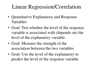
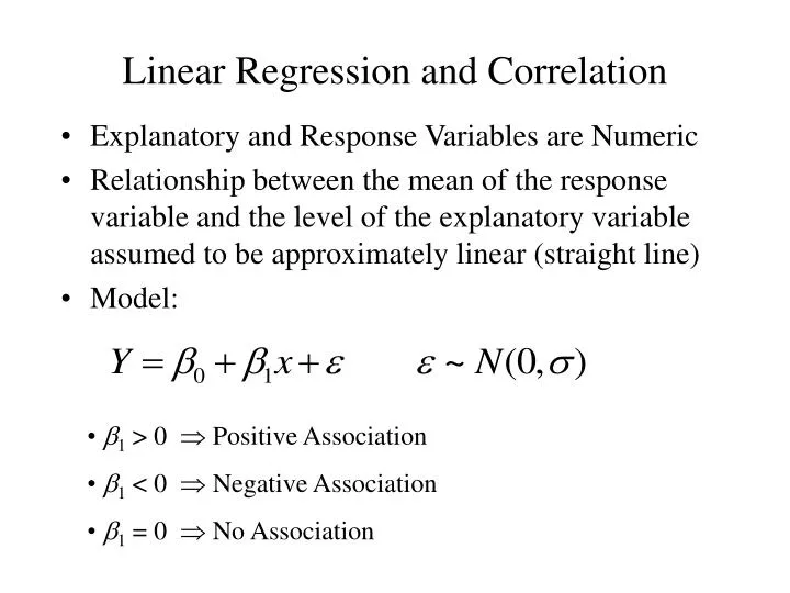
Linear Regression and Correlation • Explanatory and Response Variables are Numeric • Relationship between the mean of the response variable and the level of the explanatory variable assumed to be approximately linear (straight line) • Model: • b1 > 0 Positive Association • b1 < 0 Negative Association • b1 = 0 No Association
Least Squares Estimation of b0, b1 • b0 Mean response when x=0 (y-intercept) • b1 Change in mean response when x increases by 1 unit (slope) • b0,b1 are unknown parameters (like m) • b0+b1x Mean response when explanatory variable takes on the value x • Goal: Choose values (estimates) that minimize the sum of squared errors (SSE) of observed values to the straight-line:
Example - Pharmacodynamics of LSD • Response (y) - Math score (mean among 5 volunteers) • Predictor (x) - LSD tissue concentration (mean of 5 volunteers) • Raw Data and scatterplot of Score vs LSD concentration: Source: Wagner, et al (1968)
Example - Pharmacodynamics of LSD (Column totals given in bottom row of table)
Inference Concerning the Slope (b1) • Parameter: Slope in the population model(b1) • Estimator: Least squares estimate: • Estimated standard error: • Methods of making inference regarding population: • Hypothesis tests (2-sided or 1-sided) • Confidence Intervals
2-Sided Test H0: b1 = 0 HA: b1 0 1-sided Test H0: b1 = 0 HA+: b1> 0 or HA-: b1< 0 Hypothesis Test for b1
(1-a)100% Confidence Interval for b1 • Conclude positive association if entire interval above 0 • Conclude negative association if entire interval below 0 • Cannot conclude an association if interval contains 0 • Conclusion based on interval is same as 2-sided hypothesis test
Example - Pharmacodynamics of LSD • Testing H0: b1 = 0 vs HA: b1 0 • 95% Confidence Interval for b1 :
Confidence Interval for Mean When x=x* • Mean Response at a specific level x* is • Estimated Mean response and standard error (replacing unknown b0 and b1 with estimates): • Confidence Interval for Mean Response:
Prediction Interval of Future Response @ x=x* • Response at a specific level x* is • Estimated response and standard error (replacing unknown b0 and b1 with estimates): • Prediction Interval for Future Response:
Correlation Coefficient • Measures the strength of the linear association between two variables • Takes on the same sign as the slope estimate from the linear regression • Not effected by linear transformations of y or x • Does not distinguish between dependent and independent variable (e.g. height and weight) • Population Parameter - r • Pearson’s Correlation Coefficient:
Correlation Coefficient • Values close to 1 in absolute value strong linear association, positive or negative from sign • Values close to 0 imply little or no association • If data contain outliers (are non-normal), Spearman’s coefficient of correlation can be computed based on the ranks of the x and y values • Test of H0:r = 0 is equivalent to test of H0:b1=0 • Coefficient of Determination (r2) - Proportion of variation in y “explained” by the regression on x:
Analysis of Variance in Regression • Goal: Partition the total variation in y into variation “explained” by x and random variation • These three sums of squares and degrees of freedom are: • Total (SST) DFT = n-1 • Error (SSE) DFE = n-2 • Model (SSM) DFM = 1
Analysis of Variance in Regression • Analysis of Variance - F-test • H0: b1 = 0 HA: b1 0
Example - Pharmacodynamics of LSD • Total Sum of squares: • Error Sum of squares: • Model Sum of Squares:
Example - Pharmacodynamics of LSD • Analysis of Variance - F-test • H0: b1 = 0 HA: b1 0
Multiple Regression • Numeric Response variable (Y) • p Numeric predictor variables • Model: Y = b0 + b1x1 + + bpxp + e • Partial Regression Coefficients: bi effect (on the mean response) of increasing the ith predictor variable by 1 unit, holding all other predictors constant
Example - Effect of Birth weight on Body Size in Early Adolescence • Response: Height at Early adolescence (n =250 cases) • Predictors (p=6 explanatory variables) • Adolescent Age (x1, in years -- 11-14) • Tanner stage (x2, units not given) • Gender (x3=1 if male, 0 if female) • Gestational age (x4, in weeks at birth) • Birth length (x5, units not given) • Birthweight Group (x6=1,...,6 <1500g (1), 1500-1999g(2), 2000-2499g(3), 2500-2999g(4), 3000-3499g(5), >3500g(6)) Source: Falkner, et al (2004)
Least Squares Estimation • Population Model for mean response: • Least Squares Fitted (predicted) equation, minimizing SSE: • All statistical software packages/spreadsheets can compute least squares estimates and their standard errors
Analysis of Variance • Direct extension to ANOVA based on simple linear regression • Only adjustments are to degrees of freedom: • DFM = p DFE= n-p-1
Testing for the Overall Model - F-test • Tests whether any of the explanatory variables are associated with the response • H0: b1==bp=0 (None of the xs associated with y) • HA: Not all bi = 0
Example - Effect of Birth weight on Body Size in Early Adolescence • Authors did not print ANOVA, but did provide following: • n=250 p=6 R2=0.26 • H0: b1==b6=0 • HA: Not all bi = 0
Testing Individual Partial Coefficients - t-tests • Wish to determine whether the response is associated with a single explanatory variable, after controlling for the others • H0: bi = 0 HA: bi 0 (2-sided alternative)
Example - Effect of Birth weight on Body Size in Early Adolescence Controlling for all other predictors, adolescent age, Tanner stage, and Birth length are associated with adolescent height measurement
Testing for the Overall Model - F-test • Tests whether any of the explanatory variables are associated with the response • H0: b1==bp=0 (None of Xs associated with Y) • HA: Not all bi = 0 The P-value is based on the F-distribution with p numerator and (n-p-1) denominator degrees of freedom
Comparing Regression Models • Conflicting Goals: Explaining variation in Y while keeping model as simple as possible (parsimony) • We can test whether a subset of p-g predictors (including possibly cross-product terms) can be dropped from a model that contains the remaining g predictors. H0: bg+1=…=bp =0 • Complete Model: Contains all k predictors • Reduced Model: Eliminates the predictors from H0 • Fit both models, obtaining the Error sum of squares for each (or R2 from each)
Comparing Regression Models • H0: bg+1=…=bp = 0 (After removing the effects of X1,…,Xg, none of other predictors are associated with Y) • Ha: H0 is false P-value based on F-distribution with p-g and n-p-1 d.f.
Models with Dummy Variables • Some models have both numeric and categorical explanatory variables (Recall gender in example) • If a categorical variable has k levels, need to create k-1 dummy variables that take on the values 1 if the level of interest is present, 0 otherwise. • The baseline level of the categorical variable for which all k-1 dummy variables are set to 0 • The regression coefficient corresponding to a dummy variable is the difference between the mean for that level and the mean for baseline group, controlling for all numeric predictors
Example - Deep Cervical Infections • Subjects - Patients with deep neck infections • Response (Y) - Length of Stay in hospital • Predictors: (One numeric, 11 Dichotomous) • Age (x1) • Gender (x2=1 if female, 0 if male) • Fever (x3=1 if Body Temp > 38C, 0 if not) • Neck swelling (x4=1 if Present, 0 if absent) • Neck Pain (x5=1 if Present, 0 if absent) • Trismus (x6=1 if Present, 0 if absent) • Underlying Disease (x7=1 if Present, 0 if absent) • Respiration Difficulty (x8=1 if Present, 0 if absent) • Complication (x9=1 if Present, 0 if absent) • WBC > 15000/mm3(x10=1 if Present, 0 if absent) • CRP > 100mg/ml (x11=1 if Present, 0 if absent) Source: Wang, et al (2003)
Example - Weather and Spinal Patients • Subjects - Visitors to National Spinal Network in 23 cities Completing SF-36 Form • Response - Physical Function subscale (1 of 10 reported) • Predictors: • Patient’s age (x1) • Gender (x2=1 if female, 0 if male) • High temperature on day of visit (x3) • Low temperature on day of visit (x4) • Dew point (x5) • Wet bulb (x6) • Total precipitation (x7) • Barometric Pressure (x7) • Length of sunlight (x8) • Moon Phase (new, wax crescent, 1st Qtr, wax gibbous, full moon, wan gibbous, last Qtr, wan crescent, presumably had 8-1=7 dummy variables) Source: Glaser, et al (2004)
Analysis of Covariance • Combination of 1-Way ANOVA and Linear Regression • Goal: Comparing numeric responses among k groups, adjusting for numeric concomitant variable(s), referred to as Covariate(s) • Clinical trial applications: Response is Post-Trt score, covariate is Pre-Trt score • Epidemiological applications: Outcomes compared across exposure conditions, adjusted for other risk factors (age, smoking status, sex,...)
Nonlinear Regression • Theory often leads to nonlinear relations between variables. Examples: • 1-compartment PK model with 1st-order absorption and elimination • Sigmoid-Emax S-shaped PD model
Example - P24 Antigens and AZT • Goal: Model time course of P24 antigen levels after oral administration of zidovudine • Model fit individually in 40 HIV+ patients: • where: • E(t) is the antigen level at time t • E0 is the initial level • A is the coefficient of reduction of P24 antigen • koutis the rate constant of decrease of P24 antigen Source: Sasomsin, et al (2002)
Example - P24 Antigens and AZT • Among the 40 individuals who the model was fit, the means and standard deviations of the PK “parameters” are given below: • Fitted Model for the “mean subject”
Example - MK639 in HIV+ Patients • Response: Y = log10(RNA change) • Predictor: x = MK639 AUC0-6h • Model: Sigmoid-Emax: • where: • b0 is the maximum effect (limit as x) • b1 is the x level producing 50% of maximum effect • b2 is a parameter effecting the shape of the function Source: Stein, et al (1996)
Example - MK639 in HIV+ Patients • Data on n = 5 subjects in a Phase 1 trial: • Model fit using SPSS (estimates slightly different from notes, which used SAS)
Data Sources • Wagner, J.G., G.K. Aghajanian, and O.H. Bing (1968). “Correlation of Performance Test Scores with Tissue Concentration of Lysergic Acid Diethylamide in Human Subjects,” Clinical Pharmacology and Therapeutics, 9:635-638.