Download
1 / 49
500 likes | 681 Views
Correlation, linear regression. Scatterplot Relationship between two continouous variables. Scatterplot Relationship between two continouous variables. Scatterplot Other examples. Example II.

E N D
Example II. • Imagine that 6 students are given a battery of tests by a vocational guidance counsellor with the results shown in the following table: • Variables measured on the same individuals are often related to each other.
Let us draw a graph called scattergram to investigate relationships. • Scatterplots show the relationship between two quantitative variables measured on the same cases. • In a scatterplot, we look for the direction, form, and strength of the relationship between the variables. The simplest relationship is linear in form and reasonably strong. • Scatterplots also reveal deviations from the overall pattern.
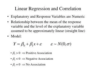
Creating a scatterplot When one variable in a scatterplot explains or predicts the other, place it on the x-axis. Place the variable that responds to the predictor on the y-axis. If neither variable explains or responds to the other, it does not matter which axes you assign them to.
Possible relationships negative correlation positive correlation no correlation
Correlation is a numerical measure of the strength of a linear association. The formula for coefficient of correlation treats x and y identically. There is no distinction between explanatory and response variable. Let us denote the two samples by x1,x2,…xn and y1,y2,…yn , the coefficient of correlation can be computed according to the following formula Describing linear relationship with number: the coefficient of correlation (r).Also called Pearson coefficient of correlation
Karl Pearson • Karl Pearson (27 March 1857 – 27 April 1936) established the discipline of mathematical statistics. http://en.wikipedia.org/wiki/Karl_Pearson
Properties of r • Correlations are between -1 and +1; the value of r is always between -1 and 1, either extreme indicates a perfect linear association. -1r 1. • a) If r is near +1 or -1 we say that we have high correlation. • b) If r=1, we say that there is perfect positive correlation. If r= -1, then we say that there is a perfect negative correlation. • c) A correlation of zero indicates the absence of linear association. When there is no tendency for the points to lie in a straight line, we say that there is no correlation (r=0) or we have low correlation (r is near 0 ).
Calculated values of r positive correlation, r=0.9989 negative correlation, r=-0.9993 no correlation, r=-0.2157
ScatterplotOther examples r=0.873 r=0.018
Correlation and causation a correlation between two variables does not show that one causes the other.
Correlation by eyehttp://onlinestatbook.com/stat_sim/reg_by_eye/index.html This applet lets you estimate the regression line and to guess the value of Pearson's correlation. Five possible values of Pearson's correlation are listed. One of them is the correlation for the data displayed in the scatterplot. Guess which one it is. To see the correct value, click on the "Show r" button.
Effect of outliers • Even a single outlier can change the correlation substantially. • Outliers can create • an apparently strong correlation where none would be found otherwise, • or hide a strong correlation by making it appear to be weak. r=-0.21 r=0.74 r=0.998 r=-0.26
Correlation and linearity • Two variables may be closely related and still have a small correlation if the form of the relationship is not linear. r=2.8 E-15 (=0.0000000000000028) r=0.157
Correlation and linearity Four sets of data with the same correlation of 0.816 http://en.wikipedia.org/wiki/Correlation_and_dependence
Coefficient of determination The square of the correlation coefficient multiplied by 100 is called the coefficient of determination. It shows the percentages of the total variation explained by the linear regression. Example. The correlation between math aptitude and language aptitude was found r =0,9989. The coefficient of determination, r2 = 0.917 . So 91.7% of the total variation of Y is caused by its linear relationship with X .
When is a correlation „high”? What is considered to be high correlation varies with the field of application. The statistician must decide when a sample value of r is far enough from zero, that is, when it is sufficiently far from zero to reflect the correlation in the population.
Testing the significance of the coefficient of correlation The statistician must decide when a sample value of r is far enough from zero to be significant, that is, when it is sufficiently far from zero to reflect the correlation in the population. (details: lecture 8.)
Prediction based on linear correlation: the linear regression When the form of the relationship in a scatterplot is linear, we usually want to describe that linear form more precisely with numbers. We can rarely hope to find data values lined up perfectly, so we fit lines to scatterplots with a method that compromises among the data values. This method is called the method of least squares. The key to finding, understanding, and using least squares lines is an understanding of their failures to fit the data; the residuals.
Prediction based on linear correlation: the linear regression A straight line that best fits the data: y=bx + a or y= a + bx is called regression line Geometrical meaning of a and b. b: is called regression coefficient, slope of the best-fitting line or regression line; a: y-intercept of the regression line. The principle of finding the values a and b, given x1,x2,…xn and y1,y2,…yn. Minimising the sum of squared residuals, i.e. Σ( yi-(a+bxi) )2 → min
Residuals, example 3. (x1,y1) y1-(b*x1+a) b*x1+a y2-(b*x2+a) y6-(b*x6+a)
Equation of regression line for the data of Example 1. • y=1.016·x+15.5the slope of the line is 1.016 • Prediction based on the equation: what is the predicted score for language for a student having 400 points in math? • ypredicted=1.016 ·400+15.5=421.9
Computation of the correlation coefficient from the regression coefficient. There is a relationship between the correlation and the regression coefficient: where sx, sy are the standard deviations of the samples . From this relationship it can be seen that the sign of r and b is the same: if there exist a negative correlation between variables, the slope of the regression line is also negative .
SPSS output for the relationship between age and body mass Coefficient of correlation, r=0.018 Equation of the regression line: y=0.078x+66.040
SPSS output for the relationship between body mass at present and 3 years ago Coefficient of correlation, r=0.873 Equation of the regression line: y=0.795x+10.054
Regression using transformations Sometimes, useful models are not linear in parameters. Examining the scatterplot of the data shows a functional, but not linear relationship between data.
Example • A fast food chain opened in 1974. Each year from 1974 to 1988 the number of steakhouses in operation is recorded. • The scatterplot of the original data suggests an exponential relationship between x (year) and y (number of Steakhouses) (first plot) • Taking the logarithm of y, we get linear relationship (plot at the bottom)
Performing the linear regression procedure to x and log (y) we get the equation log y = 2.327 + 0.2569 x that is y = e2.327 + 0.2569 x=e2.327e0.2569x= 1.293e0.2569x is the equation of the best fitting curve to the original data.
y = 1.293e0.2569x log y = 2.327 + 0.2569 x
Types of transformations Some non-linear models can be transformed into a linear model by taking the logarithms on either or both sides. Either 10 base logarithm (denoted log) or natural (base e) logarithm(denoted ln) can be used. If a>0 and b>0, applying a logarithmic transformation to the model
Exponential relationship ->take log y Model: y=a*10bx Take the logarithm of both sides: lg y =lga+bx so lg y is linear in x
Logarithm relationship ->take log x Model: y=a+lgx so y is linear in lg x
Power relationship ->take log x and log y Model: y=axb Take the logarithm of both sides: lg y =lga+b lgx so lgy is linear in lg x
Log10 base logarithmic scale 10 9 8 7 6 5 4 3 2 1
Logarithmic papers log-log paper Semilogarithmic paper
Reciprocal relationship ->take reciprocal of x Model: y=a +b/x y=a +b*1/x so y is linear in 1/x
Example 2. EL HADJ OTHMANE TAHA és mtsai: Osteoprotegerin: a regulátor, a protektor és a marker. Orvosi Hetilap 2008 ■ 149. évfolyam, 42. szám ■ 1971–1980.
Useful WEB pages • http://davidmlane.com/hyperstat/desc_biv.html • http://onlinestatbook.com/stat_sim/reg_by_eye/index.html • http://www.youtube.com/watch?v=CSYTZWFnVpg&feature=related • http://www.statsoft.com/textbook/basic-statistics/#Correlationsb • http://people.revoledu.com/kardi/tutorial/Regression/NonLinear/LogarithmicCurve.htm • http://www.physics.uoguelph.ca/tutorials/GLP/
The origin of the word „regression”. Galton: Regression towards mediocrity in hereditary stature. Journal of the Anthropological Institute 1886 Vol.15, 246-63