Download
1 / 24
240 likes | 420 Views
Correlation and Linear Regression. Evaluating Relations Between Interval Level Variables. Up to now you have learned to evaluate differences between the means of different groups, as well as evaluate relations between variables that are either Nominal or Ordinal.

E N D
Evaluating Relations Between Interval Level Variables • Up to now you have learned to evaluate differences between the means of different groups, as well as evaluate relations between variables that are either Nominal or Ordinal. • In this section you will learn how to evaluate relations between variables measured at the Interval level. As an aside, these methods will under certain conditions also allow you to evaluate Nominal or Ordinal variables as they pertain to an Interval level variable. • We can use correlation analysis to evaluate bivariate relationships (only two variables). We can use regression analysis to evaluate bivariate and multivariate relationships (more than two variables).
Definition of Correlation and Regression Analysis • Correlation analysis produces a measure of association known as Pearson’s correlation coefficient (r) which gauges the strength and direction of a relation between two variables. • Regression analysis produces a statistic, the regression coefficient () that estimates the size of the effect of an independent variable on the dependent variable. • The next slide shows the relationship between two Interval level variables, the percentage of a state’s population having a high school diploma (independent variable) and the percentage of the eligible population that voted in the 2006 elections (dependent variable). We are positing theoretically here that education affects the propensity to vote. • The type of plot given on the next slide is called a “scatter plot.”
Dependent Variable Independent Variable The plot shows that increasing education produces increasing turnout. Is this relationship positive or negative? What would it look like if it were negative? Is the relationship perfect? What would a perfect relationship look like? What would no relationship look like?
Pearson’s Correlation Coefficient (r) • Pearson’s correlation coefficient, which is symbolized by the lower case italicized r, evaluates both the direction and magnitude of the relationship between two Interval level variables. • It is calculated: • Where x is the values of the independent variable, y is the values of the dependent variable, x bar is the mean of x, y bar is the mean of y, and n is the number of observations.
Interpreting Pearson’s r • Pearson’s r ranges from -1 to 1. • When Pearson’s r is zero, there is no relationship. • When Pearson’s r is -1, there is a perfect negative relationship. • When Pearson’s r is 1, there is a perfect positive relationship. • The sign on Pearson’s r indicates the direction of the relationship. • The magnitude of Pearson’s r indicates the strength of the relationship. • It is important to note that Pearson’s r is a symmetrical measure of association. As such, the statistic cannot tell us which variable is causing which. It simply says there is or is not a relationship. We must use theory to posit a direction.
Bivariate Regression • Regression analysis allows us to put a finer point on interpretation of relationships. Using regression we can tell precisely how much the independent variable affects the dependent variable. • Consider the following Excel spreadsheet which depicts the hypothetical relationship between the percent of votes given to a political party in a proportional representation system and the percent of seats the party achieves in the legislature. • Fair Representation Spreadsheet
Evaluating the Fair Representation Model • If an electoral system is “fair,” then this would imply that a party would get the same proportion of seats in the legislature as the proportion of the votes received in the electorate. • The theoretical model says that when it receives zero votes, then it should receive zero seats. Similarly, when it receives 100 percent of the votes it should receive 100 percent of the seats. This relationship is positive, and if perfect can be represented by a line running from 0 in the left corner to 1 in the right corner. • We can represent this as a regression line using the algebraic equation:
Again, • From high school algebra, the intercept for this line (0) is zero. The intercept represents the proportion of the seats obtained when the proportion of votes is zero. • From high school algebra, the slope of the line (1) represents the change in the percent seats obtained for a one percent change in the number of votes. • If the slope of the line is positive, then the relationship is positive. If negative, then the relationship is negative. • Any deviation of the intercept from zero or the slope from one would indicate unfair representation.
Suppose we change the intercept of the regression line from 0 to 0.1. How do we interpret the result. Look again at the graph. When the percent votes obtained is 10 percent, the party still gets none of the seats. • Suppose we change the slope of the regression line from 1 to .9. How do we interpret the result. Look again at the graph. • Suppose there is an intercept of 10 and a slope of 0.9. What would be the prediction of our model for the proportion of seats a party gets when it has fifty percent of the votes.
Our estimated intercept (0) and slope (1) are subject to sampling error in precisely the same way as we described earlier for a mean or a difference in means. That is, these two statistics will vary from sample to sample. • Because the intercept and slope are subject to sampling error, we will want to test hypotheses that the population coefficients could be different than those we estimate in the sample. • As before, we do this using either a confidence interval approach or a p-value approach. • We know that the true value of in the population is equal to the sample estimate within the bounds of the standard error. For example, a 95 percent boundary would be: • We can also compute a t-statistic for either the intercept or the slope using
The regression line we saw in the spreadsheet indicates a perfect relationship. • Of course, it is unlikely that the relationship in the real world will be perfect. Therefore, we will often observe error. That is, This equation is represented in the second graph in the spreadsheet.
Goodness of Fit for a Regression • The amount of error that we introduced here implies the goodness of the fit of the theoretical model. The goodness of fit of a regression. • The most commonly used goodness of fit statistic for linear regression is R2. This statistic measures the closeness of the actual observations to the model predictions (i.e., the regression line). • The value of R2 ranges from 0 to 1. Zero indicates no relationship; the line is horizontal. One indicates a perfect relationship. All of the observed values fall exactly on the line. • R2 is a PRE measure of fit. It evaluates how much better we can predict outcomes knowing the regression results, relative to what we would predict with just the mean of the data.
R2 is calculated by using the sum of the squared distances of the observed values from the regression line and then comparing this to the sum of the squared distances when using the mean as the prediction. • It is calculated: • Because R2 always increases as you add new variables to a regression equation, adjusted R2 is often used in multiple regression. It is calculated:
Multiple Regression • Multiple Regression calculates the independent effect of multiple variables on the dependent variable. • The intercept is interpreted in the same way as above. When all of the independent variables are held a zero, the value of y is 0 . • The various slope coefficients are now called partial slope coefficients. • The partial slope coefficients are interpreted for each one unit change in X, the value of y changes by units, holding all of the other X constant. • For example, consider the following table from Pollack. Let’s interpret the results from this analysis.
Regression with Dummy Variables • A dummy variable is a variable which is switched on (has value 1) when a condition is present and switched off when the condition is not present. • For example, in the preceding analysis, the variable South is coded 1 when a respondent is from the South, and 0 when the respondent is not from the South. With a single dummy variable in a multiple regression equation, the coefficient for that variable represents the shift in the regression intercept. • For example, from the preceding table, the implied regression equation is: • We can interpret this result as follows. With South switched off, holding education constant at some value voter turnout is 3.70+0.74*Education. With South switched on, holding education constant voter turnout is (3.70-7.57=-3.87)+0.74*Education.
Dummy Variable Regression • We can do the same thing we did earlier in testing the difference in means using dummy variable regression. • For example, consider the following table which tests for whether the mean of South is the same as the mean of Non-South in voter turnout.
We can also test whether multiple group means are the same using multiple regression. For example, consider the following table.
Here the intercept represents all respondents which are not Northeast, West, and South. The mean of this group is 48.73. The mean for Northeast is 48.73-2.69=46.04. However, we can’t be confident that it is not equal to the intercept, because the t-statistic is about -1. The mean for West is 48.73-4.36=44.37. However, again we can’t be confident it is not equal to the intercept, because the t-statistic is about -1.69 The mean for South is 48.73-11.82=36.91. Here we can be very confident that South is different. Why?
Interaction Effects • Consider another example in which we have one interval level variable and one dummy variable on the right side of a multiple regression equation. • Let the dependent variable be “Liking for Madonna” on a 0-100 thermometer. • Let the interval level variable be Age. • Let the dummy variable be gender, coded 1 for men and zero for women. Then we can represent this relationship as follows. • Suppose, however, that we hypothesize that Liking for Madonna depends on both Age and being a Man, but that the effect of Age on Liking for Madonna also varies by gender. In other words, old men like Madonna differently than old women. • Then we might want to represent the relationship interactively.
Let’s explore the implications of the Madonna example using a spreadsheet. • Using an interactive model, the effect for the dummy (2)is additive with the intercept (0). In other words, the intercept for the model becomes (0 +2) when Man is present. • The effect for the interaction term is additive with the slope coefficient. In other words, the slope for the model becomes (1+3) when man is present.
A more serious example. What is the intercept for the multiple regression model below when political knowledge is not high? It is 4.33. What is the slope for partisanship when political knowledge is not high. It is -0.70?What is the intercept for the multiple regression when political knowledge is high? It is 4.33+1.50=5.83. What is the slope for partisanship when political knowledge is high? It is -0.70-0.76=-1.46