Z-scores and Correlations

1. Z-scores and Correlations Lecture 6, Psych 350 - R. Chris Fraleyhttp://www.yourpersonality.net/psych350/fall2012/

2. Announcements • No lab on Wed this week • No lecture next week • Email TA about zero-acquaintance data; working with it on Friday

3. Answering Descriptive Questions in Multivariate Research • When we are studying more than one variable, we are typically asking one (or more) of the following two questions: • How does a person’s score on the first variable compare to his or her score on a second variable? • How do scores on one variable vary as a function of scores on a second variable?

4. Making Sense of Scores • Let’s work with this first issue for a moment. • Let’s assume we have Marc’s scores on his first two Psych 350 exams. • Marc has a score of 50 on his first exam and a score of 50 on his second exam. • On which exam did Marc do best?

5. Example 1 • In one case, Marc’s exam score is 10 points above the mean • In the other case, Marc’s exam score is 10 points below the mean • In an important sense, we must interpret Marc’s grade relative to the average performance of the class Exam1 Exam2 Mean Exam1 = 40 Mean Exam2 = 60

6. Example 2 • Both distributions have the same mean (40), but different standard deviations (10 vs. 20). • In one case, Marc is performing better than almost 95% of the class. In the other, he is performing better than approximately 68% of the class. • Thus, how we evaluate Marc’s performance depends on how much spread or variability there is in the exam scores. Exam1 Exam2

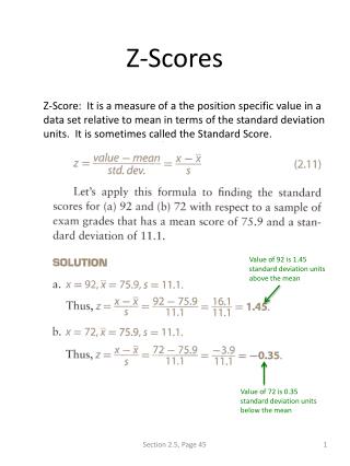
7. Standard Scores • In short, what we would like to do is express Marc’s score for any one exam with respect to (a) how far he is from the average score in the class and (b) the variability of the exam scores. • how far a person is from the mean: • (X – M) • variability in scores: • SD

8. Standard Scores • Standardized scores, or z-scores, provide a way to express how far a person is from the mean, relative to the variation of the scores. • (1) Subtract the person’s score from the mean. (2) Divide that difference by the standard deviation. ** This tells us how far a person is from the mean, in the metric of standard deviation units ** Z = (X – M)/SD

9. Example 1 Marc’s z-score on Exam1: z = (50 - 40)/10 = 1 (one SD above the mean) Marc’s z-score on Exam2 z = (50 - 60)/10 = -1 (one SD below the mean) Exam1 Exam2 Mean Exam1 = 40 SD = 10 Mean Exam2 = 60 SD = 10

10. Example 2 An example where the means are identical, but the two sets of scores have different spreads Marc’s Exam1 Z-score Z = (50-40)/5 = 2 Marc’s Exam2 Z-score Z = (50-40)/20 = .5 Exam1 SD = 5 Exam2 SD = 20

11. Some Useful Properties of Standard Scores (1) The mean of a set of z-scores is always zero Why? If we subtract a constant, C, from each score, the mean of the scores will be off by that amount (M – C). If we subtract the mean from each score, then mean will be off by an amount equal to the mean (M – M = 0).

12. (2) The SD of a set of standardized scores is always 1 • Why? SD/SD = 1 if x = 60, M = 50 SD = 10 x 20 30 40 50 60 70 80 z -3 -2 -1 0 1 2 3

13. (3) The distribution of a set of standardized scores has the same shape as the unstandardized (raw) scores

14. A “Normal” Distribution 0.4 0.3 0.2 0.1 0.0 -4 -2 0 2 4 SCORE • The “normalization” (mis)interpretation

15. Some Useful Properties of Standard Scores (4) Standard scores can be used to compute easily centile scores: the proportion of people with scores less than or equal to a particular score.

16. The area under a normal curve 50% 34% 34% 14% 14% 2% 2%

17. Some Useful Properties of Standard Scores (5) Z-scores provide a way to “standardize” different metrics (i.e., metrics that differ in variation or meaning). Different variables expressed as z-scores can be interpreted on the same metric (the z-score metric). (Each score comes from a distribution with the same mean [zero] and the same standard deviation [1].)

19. Correlations in Personality Research • Many research questions that are addressed in personality psychology are concerned with the relationship between two or more variables.

20. Some examples • How does dating/marital satisfaction vary as a function of personality traits, such as emotional stability? • Are people who are relatively sociable as children also likely to be relatively sociable as adults? • What is the relationship between individual differences in violent video game playing and aggressive behavior in adolescents?

21. Graphic presentation • Many of the relationships we’ll focus on in this course are of the linear variety. • The relationship between two variables can be represented as a line. aggressive behavior violent video game playing

22. Linear relationships can be negative or positive. aggressive behavior aggressive behavior violent game playing violent game playing

23. How do we determine whether there is a positive or negative relationship between two variables?

24. Scatter plots One way of determining the form of the relationship between two variables is to create a scatter plot or a scatter graph. The form of the relationship (i.e., whether it is positive or negative) can often be seen by inspecting the graph. aggressive behavior violent game playing

25. How to create a scatter plot Use one variable as the x-axis (the horizontal axis) and the other as the y-axis (the vertical axis). Plot each person in this two dimensional space as a set of (x, y) coordinates.

26. How to create a scatter plot in SPSS

27. How to create a scatter plot in SPSS • Select the two variables of interest. • Click the “ok” button.

28. positive relationship negative relationship no relationship

29. Quantifying the relationship • How can we quantify the linear relationship between two variables? • One way to do so is with a commonly used statistic called the correlation coefficient (often denoted as r).

30. Some useful properties of the correlation coefficient • Correlation coefficients range between –1 and + 1. Note: In this respect, r is useful in the same way that z-scores are useful: they both use a standardized metric.

31. Some useful properties of the correlation coefficient (2) The value of the correlation conveys information about the form of the relationship between the two variables. • When r > 0, the relationship between the two variables is positive. • When r < 0, the relationship between the two variables is negative--an inverse relationship (higher scores on x correspond to lower scores on y). • When r = 0, there is no relationship between the two variables.

32. r = .80 r = -.80 r = 0

33. Some useful properties of the correlation coefficient (3) The correlation coefficient can be interpreted as the slope of the line that maps the relationship between two standardized variables. slope as rise over run

34. r = .50 takes you up .5 on y rise run moving from 0 to 1 on x

35. How do you compute a correlation coefficient? • First, transform each variable to a standardized form (i.e., z-scores). • Multiply each person’s z-scores together. • Finally, average those products across people.

36. Example

37. Why products? Important Note on 2 x 2 Matching z-scores via products

38. Important Note on 2 x 2

39. Computing Correlations in SPSS • Go to the “Analyze” menu. • Select “Correlate” • Select “Bivariate…”

40. Computing Correlations in SPSS • Select the variables you want to correlate • Shoot them over to the right-most window • Click on the “Ok” button.

41. Magnitude of correlations • When is a correlation “big” versus “small?” • Cohen’s standards: • .1 small • .3 medium • > .5 large

42. What are typical correlations in personality psychology? Typical sample sizes and effect sizes in studies conducted in personality psychology. Note. The absolute value of r was used in the calculations reported here. Data are based on articles published in the 2004 volumes of JPSP:PPID and JP.

43. A selection of effect sizes from various domains of research Note. Table adapted from Table 1 of Meyer et al. (2001).

44. Magnitude of correlations • “real world” correlations are rarely get larger than .30. • Why is this the case? • Any one variable can be influenced by a hundred other variables. To the degree to which a variable is multi-determined, the correlation between it and any one variable must be small.

45. Qualify • For the purposes of this class, I want you to describe the correlation: What is it numerically? And, qualitatively speaking, is it “zero or close to zero” (< .1), “small” (.1 to .29), “medium” (.30 to .49), or “large” (> .50).