Download

1 / 46
710 likes | 1.53k Views
Principles of Linear Pipelining. Example : Floating Point Adder Unit. Floating Point Adder Unit. This pipeline is linearly constructed with 4 functional stages. The inputs to this pipeline are two normalized floating point numbers of the form A = a x 2 p B = b x 2 q

E N D
Floating Point Adder Unit • This pipeline is linearly constructed with 4 functional stages. • The inputs to this pipeline are two normalized floating point numbers of the form A = a x 2p B = b x 2q where a and b are two fractions and p and q are their exponents. • For simplicity, base 2 is assumed
Floating Point Adder Unit • Our purpose is to compute the sum C = A + B = c x 2r = d x 2s where r = max(p,q) and 0.5 ≤ d < 1 • For example: A=0.9504 x 10³ B=0.8200 x 10² a = 0.9504 b= 0.8200 p=3 & q =2
Floating Point Adder Unit • Operations performed in the four pipeline stages are : • Compare p and q and choose the largest exponent, r = max(p,q)and compute t = |p – q| Example: r = max(p , q) = 3 t = |p-q| = |3-2|= 1
Floating Point Adder Unit • Shift right the fraction associated with the smaller exponent by t units to equalize the two exponents before fraction addition. • Example: Smaller exponent, b= 0.8200 Shift right b by 1 unit is 0.082
Floating Point Adder Unit • Perform fixed-point addition of two fractions to produce the intermediate sum fraction c, where 0 ≤ c < 1 • Example : a = 0.9504 b= 0.082 c = a + b = 0.9504 + 0.082 = 1.0324
Floating Point Adder Unit • Count the number of leading zeros (u) in fraction c and shift left c by u units to produce the normalized fraction sum d = c x 2u, with a leading bit 1. Update the large exponent s by subtracting s = r – u to produce the output exponent. • Example: c = 1.0324 , u = -1 right shift d = 0.10324 , s= r – u = 3-(-1) = 4 C = 0.10324 x 10⁴
Floating Point Adder Unit • The above 4 steps can all be implemented with combinational logic circuits and the 4 stages are: • Comparator / Subtractor • Shifter • Fixed Point Adder • Normalizer (leading zero counter and shifter)
4-STAGE FLOATING POINT ADDER p q A = a x 2 B = b x 2 a A b B Other Stages: Fraction Exponent fraction subtractor selector S1 Fraction with min(p,q) r = max(p,q) Right shifter t = |p - q| Fraction S2 adder c r Leading zero counter S3 c Left shifter r d Exponent adder S4 s d C= X + Y = d x 2s
Exponents Mantissas a b A B R R Difference=3-2=1 For example: X=0.9504*103 Y=0.8200*102 Compare exponents by subtraction Segment 1: Align mantissas 0.082 R R 3 Choose exponent Segment 2: Add mantissas S=0.9504+0.082=1.0324 Segment 3: R R 4 Adjust exponent Normalize result 0.10324 Segment 4: R R Example for floating-point adder
Classification of Pipeline Processors • There are various classification schemes for classifying pipeline processors. • Two important schemes are • Handler’s Classification • Li and Ramamurthy's Classification
Handler’s Classification • Based on the level of processing, the pipelined processors can be classified as: • Arithmetic Pipelining • Instruction Pipelining • Processor Pipelining
Arithmetic Pipelining • The arithmetic logic units of a computer can be segmented for pipelined operations in various data formats. • Example : Star 100
Arithmetic Pipelining • Example : Star 100 • It has two pipelines where arithmetic operations are performed • First: Floating Point Adder and Multiplier • Second : Multifunctional • All scalar instructions • Floating point adder, multiplier and divider. • Both pipelines are 64-bit and can be split into four 32-bit at the cost of precision
Instruction Pipelining • The execution of a stream of instructions can be pipelined by overlapping the execution of current instruction with the fetch, decode and operand fetch of the subsequent instructions • It is also called instruction look-ahead
Example : 8086 • The organization of 8086 into a separate BIU and EU allows the fetch and execute cycle to overlap. This is called pipelining.
Processor Pipelining • This refers to the processing of same data stream by a cascade of processors each of which processes a specific task • The data stream passes the first processor with results stored in a memory block which is also accessible by the second processor • The second processor then passes the refined results to the third and so on.
Li and Ramamurthy's Classification • According to pipeline configurations and control strategies, Li and Ramamurthy classify pipelines under three schemes • Unifunction v/s Multi-function Pipelines • Static v/s Dynamic Pipelines • Scalar v/s Vector Pipelines
Unifunctional Pipelines • A pipeline unit with fixed and dedicated function is called unifunctional. • Example: CRAY1 (Supercomputer - 1976) • It has 12 unifunctional pipelines described in four groups: • Address Functional Units: • Address Add Unit • Address Multiply Unit
Unifunctional Pipelines • Scalar Functional Units • Scalar Add Unit • Scalar Shift Unit • Scalar Logical Unit • Population/Leading Zero Count Unit • Vector Functional Units • Vector Add Unit • Vector Shift Unit • Vector Logical Unit
Unifunctional Pipelines • Floating Point Functional Units • Floating Point Add Unit • Floating Point Multiply Unit • Reciprocal Approximation Unit
Multifunctional A multifunction pipe may perform different functions either at different times or same time, by interconnecting different subset of stages in pipeline. Example 4X-TI-ASC (Supercomputer - 1973)
4X-TI ASC It has four multifunction pipeline processors, each of which is reconfigurable for a variety of arithmetic or logic operations at different times. It is a four central processor comprised of nine units.
Multifunctional • It has • one instruction processing unit • four memory buffer units and • four arithmetic units. • Thus it provides four parallel execution pipelines below the IPU. • Any mixture of scalar and vector instructions can be executed simultaneously in four pipes.
Static Pipeline • It may assume only one functional configuration at a time • It can be either unifunctional or multifunctional • Static pipelines are preferred when instructions of same type are to be executed continuously • A unifunction pipe must be static.
Dynamic pipeline • It permits several functional configurations to exist simultaneously • A dynamic pipeline must be multi-functional • The dynamic configuration requires more elaborate control and sequencing mechanisms than static pipelining
Scalar Pipeline • It processes a sequence of scalar operands under the control of a DO loop • Instructions in a small DO loop are often prefetched into the instruction buffer. • The required scalar operands are moved into a data cache to continuously supply the pipeline with operands • Example: IBM System/360 Model 91
IBM System/360 Model 91 • In this computer, buffering plays a major role. • Instruction fetch buffering: • provide the capacity to hold program loops of meaningful size. • Upon encountering a loop which fits, the buffer locks onto the loop and subsequent branching requires less time. • Operand fetch buffering: • provide a queue into which storage can dump operands and execution units can fetch operands. • This improves operand fetching for storage-to-register and storage-to-storage instruction types.
Vector Pipelines • They are specially designed to handle vector instructions over vector operands. • Computers having vector instructions are called vector processors. • The design of a vector pipeline is expanded from that of a scalar pipeline. • The handling of vector operands in vector pipelines is under firmware and hardware control. • Example : Cray 1
Linear pipeline (Static & Unifunctional) • In a linear pipeline data flows from one stage to another and all stages are used once in a computation and it is for one functional evaluation.
Non-linear pipeline • In floating point adder, stage (2) and (4) needs a shift register. • We can use the same shift register and then there will be only 3 stages. • Then we should have a feedback from third stage to second stage. • Further the same pipeline can be used to perform fixed point addition. • A pipeline with feed-forward and/or feedback connections is called non-linear