Download
1 / 27
290 likes | 305 Views
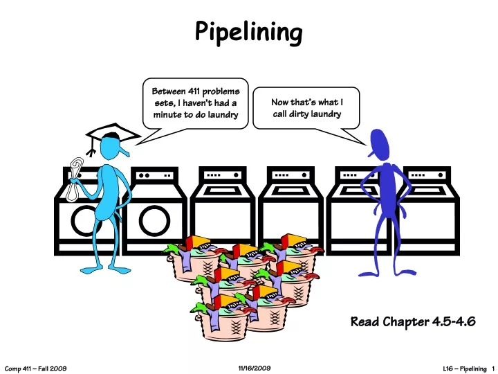
Pipelining. Between 411 problems sets, I haven’t had a minute to do laundry. Now that’s what I call dirty laundry. Read Chapter 4.5-4.6. Forget 411… Let’s Solve a “Relevant Problem”. INPUT: dirty laundry. Device: Washer Function: Fill, Agitate, Spin Washer PD = 30 mins. OUTPUT:

E N D
Pipelining Between 411 problems sets, I haven’t had a minute to do laundry Now that’s what Icall dirty laundry Read Chapter 4.5-4.6
Forget 411… Let’s Solve a “Relevant Problem” INPUT: dirty laundry Device: Washer Function: Fill, Agitate, Spin WasherPD = 30 mins OUTPUT: 4 more weeks Device: Dryer Function: Heat, Spin DryerPD = 60 mins
Everyone knows that the real reason that UNC students put off doing laundry so long is *not* because they procrastinate, are lazy, or even have better things to do. The fact is, doing laundry one load at a time is not smart. (Sorry Mom, but you were wrong about this one!) One Load at a Time Step 1: Step 2: Total = WasherPD + DryerPD = _________ mins 90
Here’s how they do laundry at Duke, the “combinational” way. (Actually, this is just an urban legend. No one at Duke actually does laundry. The butler’s all arrive on Wednesday morning, pick up the dirty laundry and return it all pressed and starched by dinner) Step 1: Step 3: Doing N Loads of Laundry Step 2: Step 4: … Total = N*(WasherPD + DryerPD) = ____________ mins N*90
UNC students “pipeline” the laundry process. That’s why we wait! Step 1: Doing N Loads… the UNC way Step 2: Step 3: … Actually, it’s more like N*60 + 30 if we account for the startup transient correctly. When doing pipeline analysis, we’re mostly interested in the “steady state” where we assume we have an infinite supply of inputs. Total = N * Max(WasherPD, DryerPD) = ____________ mins N*60
Assuming that the wash is started as soon as possible and waits (wet) in the washer until dryer is available. Even though we increase latency, it takes less time per load Recall Our Performance Measures • Latency:The delay from when an input is established until the output associated with that input becomes valid. • (Duke Laundry = _________ mins) • ( UNC Laundry = _________ mins) • Throughput: • The rate at which inputs or outputs are processed. • (Duke Laundry = _________ outputs/min) • ( UNC Laundry = _________ outputs/min) 90 120 1/90 1/60
F X P(X) H G Okay, Back to Circuits… For combinational logic: latency = tPD, throughput = 1/tPD. We can’t get the answer faster, but are we making effective use of our hardware at all times? X F(X) G(X) P(X) F & G are “idle”, just holding their outputs stable while H performs its computation
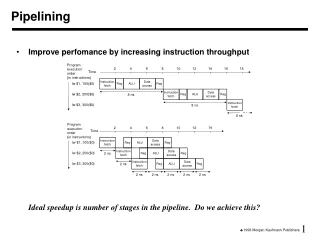
F 15 H X P(X) 25 G 20 50 1/25 worse better Pipelined Circuits use registers to hold H’s input stable! Now F & G can be working on input Xi+1 while H is performing its computation on Xi. We’ve created a 2-stage pipeline : if we have a valid input X during clock cycle j, P(X) is valid during clock j+2. Suppose F, G, H have propagation delays of 15, 20, 25 ns and we are using ideal zero-delay registers (ts = 0, tpd = 0): Pipelining uses registers to improve the throughput of combinational circuits unpipelined 2-stage pipeline latency 45 ______ throughput 1/45 ______
This is an exampleof parallelism. At any instant we are computing 2 results. F 15 Xi+1 Xi+2 Xi+3 … H X P(X) 25 F(Xi) F(Xi+1) F(Xi+2) G … 20 G(Xi) G(Xi+1) G(Xi+2) H(Xi) H(Xi+1) H(Xi+2) Pipeline Diagrams Clock cycle i i+1 i+2 i+3 Input Xi F Reg Pipeline stages G Reg H Reg The results associated with a particular set of input data moves diagonally through the diagram, progressing through one pipeline stage each clock cycle.
Pipelining Summary • Advantages: • Higher throughput than combinational system • Different parts of the logic work on different parts of the problem… • Disadvantages: • Generally, increases latency • Only as good as the *weakest* link(often called the pipeline’s BOTTLENECK) • Isn’t there a way around this “weak link” problem? This bottleneckis the onlyproblem
Step 1: Step 2: Step 3: Step 4: How do UNC students REALLY do Laundry? • They work around the bottleneck. First, they find a place with twice as many dryers as washers. • Throughput = ______ loads/min • Latency = ______ mins/load 1/30 90
Step 5: Step 1: Step 2: Step 3: Step 4: Better Yet… Parallelism We can combine interleavingand pipelining with parallelism. Throughput = _______ load/min Latency = _______ min 2/30 = 1/15 90
“Classroom Computer” There are lots of problem sets to grade, each with six problems. Students in Row 1 grade Problem 1 and then hand it back to Row 2 for grading Problem 2, and so on… Assuming we want to pipeline the grading, how do we time the passing of papers between rows? Row 1 Psets in Row 2 Row 3 Row 4 Row 5 Row 6
Controls for “Classroom Computer” Synchronous Asynchronous Teacher picks variable time interval long enough for current students to grade current set of problems. Everyone passes psets at end of interval. Teacher picks time interval long enough for worst-case student to grade toughest problem. Everyone passes psets at end of interval. Globally Timed Students raise hands when they finish grading current problem. Teacher checks every 10 secs, when all hands are raised, everyone passes psets to the row behind. Variant: students can pass when all students in a “column” have hands raised. Students grade current problem, wait for student in next row to be free, and then pass the pset back. Locally Timed
Control Structure Taxonomy Easy to design but fixed-sized interval can be wasteful (no data-dependencies in timing) Large systems lead to very complicated timing generators… just say no! Synchronous Asynchronous Central control unit tailors current time slice to current tasks. Centralized clocked FSM generates all control signals. Globally Timed Start and Finish signals generated by each major subsystem, synchronously with global clock. Each subsystem takes asynchronous Start, generates asynchronous Finish (perhaps using local clock). Locally Timed The “next big idea” for the last several decades: a lot of design work to do in general, but extra work is worth it in special cases The best way to build large systems that have independent components.
Freq MIPS = CPI Review of CPU Performance MIPS = Millions of Instructions/Second Freq = Clock Frequency, MHz CPI = Clocks per Instruction • To Increase MIPS: • 1. DECREASE CPI. • - RISC simplicity reduces CPI to 1.0. • - CPI below 1.0? State-of-the-art multiple instruction issue • 2. INCREASE Freq. • - Freq limited by delay along longest combinational path; hence • -PIPELINING is the key to improving performance.
miniMIPS Timing CLK New PC • The diagram on the left illustrates the Data Flow of miniMIPS • Wanted: longest path • Complications: • some apparent paths aren’t “possible” • functional units have variable execution times (eg, ALU) • time axis is not to scale (eg, tPD,MEM is very big!) PC+4 Fetch Inst. Control Logic Read Regs Sign Extend +OFFSET ASEL mux BSEL mux ALU Fetch data PCSEL mux WASEL mux WDSEL mux PC setup RF setup Mem setup CLK
0x80000000 PC<31:29>:J<25:0>:00 0x80000040 0x80000080 JT BT 00 PCSEL 6 5 4 3 2 1 0 PC +4 Instruction A Memory D Rs: <25:21> Rt: <20:16> WASEL J:<25:0> Rd:<15:11> 0 1 2 3 Register RA1 RA2 WD Rt:<20:16> “31” WA WA File “27” WERF RD1 RD2 WE Imm: <15:0> BSEL 1 0 RESET SEXT SEXT JT N V Z C IRQ x4 shamt:<10:6> + Control Logic “16” ASEL 0 1 2 BSEL PCSEL WDSEL BT WASEL ALUFN A B SEXT Wr ALU Wr WD R/W ALUFN Data Memory N V C Z Adr RD WERF ASEL 0 1 2 WDSEL PC+4 Where Are the Bottlenecks? • Pipelining goal: • Break LONG combinational paths • memories, ALU in separate stages
Instruction Fetch stage: Maintains PC, fetches one instruction per cycle and passes it to IF Instruction Decode/Register File stage: Decode control lines and select source operands ID/RF ALU stage: Performs specified operation, passes result to Memory stage: If it’s a lw, use ALU result as an address, pass mem data (or ALU result if not lw) to MEM Write-Back stage: writes result back into register file. ALU WB Ultimate Goal: 5-Stage Pipeline GOAL: Maintain (nearly) 1.0 CPI, but increase clock speed to barely include slowest components (mems, regfile, ALU) APPROACH: structure processor as 5-stage pipeline:
add $4, $5, $6 beq $1, $2, 40 lw $3, 30($0) jal 20000 sw $2, 20($4) miniMIPS Timing • Different instructions use various parts of the data path. 1 instr every 14 nS, 14 nS, 20 nS, 9 nS, 19 nS Program execution order Time CLK This is an example of a “Asynchronous Globally-Timed” control strategy (see Lecture 18). Such a system would vary the clock period based on the instruction being executed. This leads to complicated timing generation, and, in the end, slower systems, since it is not very compatible with pipelining! 6 nS 2 nS 2 nS 5 nS 4 nS 6 nS 1 nS Instruction Fetch Instruction Decode Register Prop Delay ALU Operation Branch Target Data Access Register Setup
Isn’t the net effect just a slower CPU? Uniform miniMIPS Timing • With a fixed clock period, we have to allow for the worse case. 1 instr EVERY 20 nS Program execution order Time CLK add $4, $5, $6 beq $1, $2, 40 lw $3, 30($0) jal 20000 sw $2, 20($4) By accounting for the “worse case” path (i.e. allowing time for each possible combination of operations) we can implement a “Synchronous Globally-Timed” control strategy. This simplifies timing generation, enforces a uniform processing order, and allows for pipelining! 6 nS 2 nS 2 nS 5 nS 4 nS 6 nS 1 nS Instruction Fetch Instruction Decode Register Prop Delay ALU Operation Branch Target Data Access Register Setup
00 00 Instruction A Memory D +4 PCEXE IREXE Rs: <25:21> Rt: <20:16> Rd:<15:11> Rt:<20:16> BSEL 1 0 Control Logic x4 BSEL WDSEL Data Memory ALUFN Wr RD 0 1 2 WDSEL Step 1: A 2-Stage Pipeline 0x80000000 PC<31:29>:J<25:0>:00 0x80000040 IF 0x80000080 JT BT PCSEL 6 5 4 3 2 1 0 PC EXE WASEL J:<25:0> 0 1 2 3 Register RA1 RA2 WD “31” WA WA File “27” WERF RD1 RD2 WE Imm: <15:0> RESET IR stands for “Instruction Register”. The superscript “EXE” denotes the pipeline stage, in which the PC and IR are used. SEXT SEXT JT N V Z C IRQ shamt:<10:6> + “16” ASEL 0 1 2 PCSEL BT WASEL A B SEXT ALU Wr WD R/W ALUFN N V C Z Adr WERF ASEL PC+4
During this, and all subsequent clocks two instructions are in various stages of execution Latency? Throughput? 2-Stage Pipe Timing • Improves performance by increasing instruction throughput.Ideal speedup is number of pipeline stages in the pipeline. Program execution order Time CLK add $4, $5, $6 beq $1, $2, 40 lw $3, 30($0) jal 20000 sw $2, 20($4) By partitioning each instruction cycle into a “fetch” stage and an “execute” stage, we get a simple pipeline. Why not include the Instruction-Decode/Register-Access time with the Instruction Fetch? You could. But this partitioning allows for a useful variant with 2-cycle loads and stores. 6 nS 2 nS 2 nS 5 nS 4 nS 6 nS 1 nS Instruction Fetch Instruction Decode Register Prop Delay ALU Operation Branch Target 2 Clock periods = 2*14 nS Data Access Register Setup 1 instrper 14 nS
This design is very similar to the multicycle CPU described in section 5.5 of the text, but with pipelining. Clock: 8 nS! 2-Stage w/2-Cycle Loads & Stores • Further improves performance, with slight increase in control complexity. Some 1st generation (pre-cache) RISC processors used this approach. Program execution order Time CLK add $4, $5, $6 beq $1, $2, 40 lw $3, 30($0) jal 20000 sw $2, 20($4) The clock rate of this variant is over twice that of our original design. Does that mean it is that much faster? 6 nS 2 nS 2 nS 5 nS 4 nS 6 nS 1 nS Instruction Fetch Instruction Decode Register Prop Delay ALU Operation Not likely. In practice, as many as 30% of instructions access memory. Thus, the effective speed up is: Branch Target Data Access Register Setup
Recall “Pipeline Diagrams” from an earlier slide. Executed on our 2-stage pipeline: i+1 i i+2 i+3 i+4 i+5 i+6 It can’t be this easy!? IF addi xor sltiu srl ... TIME (cycles) Pipeline EXE addi xor sltiu srl ... 2-Stage Pipelined Operation Consider a sequence of instructions: ... addi $t2,$t1,1 xor $t2,$t1,$t2 sltiu $t3,$t2,1 srl $t2,$t2,1 ...
00 00 00 00 +4 PCALU PCMEM PCREG A IRALU WDMEM Y WDALU IRREG B IRMEM Rs: <25:21> Rt: <20:16> BSEL 1 0 x4 Data Memory RD 0 1 2 WDSEL 0x80000000 PC<31:29>:J<25:0>:00 0x80000040 Step 2: 4-Stage miniMIPS 0x80000080 JT BT PCSEL 6 5 4 3 2 1 0 Instruction PC Memory A Treats register file as two separate devices: combinational READ, clocked WRITE at end of pipe. What other information do we have to pass down pipeline? PC instruction fields What sort of improvement should expect in cycle time? D Instruction Fetch J:<25:0> Register RA1 RA2 WA File RD1 RD2 = JT Imm: <15:0> SEXT SEXT BZ shamt:<10:6> + “16” ASEL Register 0 1 2 File BT A B ALU ALUFN (return addresses) N V C Z ALU (decoding) Wr R/W Adr WD PC+4 Rt:<20:16> Rd:<15:11> “27” “31” 0 1 2 3 WASEL (NB: SAME RF AS ABOVE!) Write Register WD WA Back WA WERF File WE
i+1 i i+2 i+3 i+4 i+5 i+6 IF addi sll andi sub ... RF addi sll andi sub ... TIME (cycles) Pipeline addi sll andi sub ... ALU addi sll andi sub WB 4-Stage miniMIPS Operation Consider a sequence of instructions: ... addi $t0,$t0,1 sll $t1,$t1,2 andi $t2,$t2,15 sub $t3,$0,$t3 ... Executed on our 4-stage pipeline: