Download

1 / 35
390 likes | 636 Views
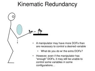
Kinematic Redundancy. A manipulator may have more DOFs than are necessary to control a desired variable What do you do w/ the extra DOFs? However, even if the manipulator has “enough” DOFs, it may still be unable to control some variables in some configurations…. Jacobian Range Space.

E N D
Kinematic Redundancy • A manipulator may have more DOFs than are necessary to control a desired variable • What do you do w/ the extra DOFs? • However, even if the manipulator has “enough” DOFs, it may still be unable to control some variables in some configurations…
Jacobian Range Space Before we think about redundancy, let’s look at the range space of the Jacobian transform: The velocity Jacobian maps joint velocities onto end effector velocities: • Space of joint velocities • This is the domain of J: • Space of end effector velocities • This is the range space of J:
Jacobian Range Space In some configurations, the range space of the Jacobian may not span the entire space of the variable to be controlled: spans if Example: a and b span this two dimensional space:
Jacobian Range Space • This is the case in the manipulator to the right: • In this configuration, the Jacobian does not span the y direction (or the z direction)
Jacobian Range Space Let’s calculate the velocity Jacobian: Joint configuration of manipulator: There is no joint velocity, , that will produce a y velocity, Therefore, you’re in a singularity.
Jacobian Singularities • In singular configurations: • does not span the space of Cartesian velocities • loses rank • Test for kinematic singularity: • If is zero, then manipulator is in a singular configuration Example:
Jacobian Singularities: Example The four singularities of the three-link planar arm:
Jacobian Singularities and Cartesian Control Cartesian control involves calculating the inverse or pseudoinverse: However, in singular configurations, the pseudoinverse (or inverse) does not exist because is undefined. As you approach a singular configuration, joint velocities in the singular direction calculated by the pseudoinverse get very large: In Jacobian transpose control, joint velocities in the singular direction (i.e. the gradient) go to zero: Where is a singular direction.
Jacobian Singularities and Cartesian Control • So, singularities are mostly a problem for Jacobian pseudoinverse control where the pseudoinverse “blows up”. • Not much of a problem for transpose control • The worst that can happen is that the manipulator gets “stuck” in a singular configuration because the direction of the goal is in a singular direction. • This “stuck” configuration is unstable – any motion away from the singular configuration will allow the manipulator to continue on its way.
Jacobian Singularities and Cartesian Control One way to get the “best of both worlds” is to use the “dampled least squares inverse” – aka the singularity robust (SR) inverse: • Because of the additional term inside the inversion, the SR inverse does not blow up. • In regions near a singularity, the SR inverse trades off exact trajectory following for minimal joint velocities. • BTW, another way to handle singularities is simply to avoid them – this method is preferred by many • More on this in a bit…
Manipulability Ellipsoid Can we characterize how close we are to a singularity? Yes – imagine the possible instantaneous motions are described by an ellipsoid in Cartesian space. Can’t move much this way Can move a lot this way
Manipulability Ellipsoid The manipulability ellipsoid is an ellipse in Cartesian space corresponding to the twists that unit joint velocities can generate: A unit sphere in joint velocity space Project the sphere into Cartesian space The space of feasible Cartesian velocities
Manipulability Ellipsoid • You can calculate the directions and magnitudes of the principle axes of the ellipsoid by taking the eigenvalues and eigenvectors of • The lengths of the axes are the square roots of the eigenvalues • Yoshikawa’s manipulability measure: • You try to maximize this measure • Maximized in isotropic configurations • This measures the volume of the ellipsoid
Manipulability Ellipsoid • Another characterization of the manipulability ellipsoid: the ratio of the largest eigenvalue to the smallest eigenvalue: • Let be the largest eigenvalue and let be the smallest. • Then the condition number of the ellipsoid is: • The closer to one the condition number, the more isotropic the ellispoid is.
Manipulability Ellipsoid Isotropic manipulability ellipsoid NOT isotropic manipulability ellipsoid
Force Manipulability Ellipsoid You can also calculate a manipulability ellipsoid for force: A unit sphere in the space of joint torques The space of feasible Cartesian wrenches
Manipulability Ellipsoid • Principle axes of the force manipulability ellipsoid: the eigenvalues and eigenvectors of: • has the same eigenvectors as : • But, the eigenvalues of the force and velocity ellipsoids are reciprocals: • Therefore, the shortest principle axes of the velocity ellipsoid are the longest principle axes of the force ellipsoid and vice versa…
Velocity and force manipulability are orthogonal! Force ellipsoid Velocity ellipsoid • This is known as force/velocity duality • You can apply the largest forces in the same directions that your max velocity is smallest • Your max velocity is greatest in the directions where you can only apply the smallest forces
Manipulability Ellipsoid: Example Solve for the principle axes of the manipulability ellipsoid for the planar two link manipulator with unit length links at Principle axes:
Kinematic redundancy • A general-purpose robot arm frequently has more DOFs than are strictly necessary to perform a given function • in order to independently control the position of a planar manipulator end effector, only two DOFs are strictly necessary • If the manipulator has three DOFs, then it is redundant w.r.t. the task of controlling two dimensional position. • In order to independently control end effector position in 3-space, you need at least 3 DOFs • In order to independently control end effector position and orientation, at least 6 DOFs are needed (they have to be configured right, too…)
Kinematic redundancy • The local redundancy of an arm can be understood in terms of the local Jacobian • The manipulator controls a number of Cartesian DOFs equal to the number of independent rows in the Jacobian Since there are two independent rows, you can control two Cartesian DOFs independently (m=2) You use three joints to control two Cartesian DOFs (n=3) Since the number of independent Cartesian directions is less than the number of joints, (m<n), this manipulator is redundant w.r.t. the task of controlling those Cartesian directions.
Kinematic redundancy • What does this redundant space look like? • At first glance, you might think that it’s linear because the Jacobian is linear • But, the Jacobian is only locally linear • The dimension of the redundant space is the number of joints – the number of independent Cartesian DOFs: n-m. • For the three link planar arm, the redundant space is a set of one dimensional curves traced through the three dimensional joint space. • Each curve corresponds to the set of joint configurations that place the end effector in the same position. Redundant manifolds in joint space
Kinematic redundancy • Joint velocities in redundant directions causes no motion at the end effector • These are internal motions of the manipulator. Redundant joint velocities satisfy this equation: the null space of Compare to the range space of : Redundant manifolds in joint space
Null space and Range space Joint space Cartesian space You can’t generate these motions • Null space • Motions in the null space are internal motions Range space
Null space and Range space Degree of manipulability: Degree of redundancy:
Null space and Range space • As the manipulator moves to new configurations, the degree of manipulability may temporarily decrease – these are the singular configurations. • There is a corresponding increase in degree of redundancy.
Null space and Range space Remember the Jacobian’s application to statics:
Null space and Range space in the Force Domain • A Cartesian force cannot generate joint torques in the joint velocity null space. • …
Doing Things in the Redundant Joint Space • Motions in the redundant space do not affect the position of the end effector. • Since they don’t change end effector position, is there something we would like to do in this space? • Optimize kinematic manipulability? • Stay away from obstacles? • Something else?
Doing Things in the Redundant Joint Space • Assume that you are given a joint velocity, , you would like to achieve while also achieving a desired end effector twist, • Required objective: • Desired objective: Minimize subject to : Use lagrange multiplier method:
Doing Things in the Redundant Joint Space Homogeneous part of the solution • Null space projection matrix: • This matrix projects an arbitrary vector into the null space of J • This makes it easy to do things in the redundant space – just calculate what you would like to do and project it into the null space.
Things You Might do in the Null Space Avoid kinematic singularities: • Calculate the gradient of the manipulability measure: • Project into null space: Avoid joint limits: • Calculate a gradient of the squared distance from a joint limit: • Project into null space: • where is the joint configuration at the center of the joints • and is the current joint position
Things You Might do in the Null Space obstacle Avoid kinematic obstacles: • Consider a set of control points (nodes) on the manipulator: • Move all nodes away from the object: • Project desired motion into joint space: • Project into null space: