Download
1 / 15
170 likes | 393 Views
Kinematic Equations. New equations and how to use them!. Kinematics – Effect of Motion Study and description of motion – without regard to the cause. Dynamics – Cause of Motion. Definitions. Equations of motion

E N D
Kinematic Equations New equations and how to use them!
Kinematics – Effect of MotionStudy and description of motion – without regard to the cause. Dynamics – Cause of Motion Definitions
Equations of motion Based on the fundamental definitions of average velocity and average acceleration: Kinematic Equations Plugging in def of Δ Arithmetic Mean
Our variables • There are 5 basic variables that are used in any motion-related calculation: • Initial Velocity = v0orvi • Final Velocity = vorvf • Acceleration = a • Displacement = Δx • Time = t • Bold face indicates a vector • Each of the kinematic equations will use 4 of these 5 variables
How far does an object travel during uniformly accelerated motion? What can we determine? Start Rearrange… Substitute…
What can we determine? Continue Rearrange… To… Substitute… Distribute Δt… Combine like terms…
Can we relate v, a, & Δx without a time variable? What can we determine? Start Rearrange… Substitute into… To get..
What can we determine? Start Substitute… To get.. Multiply binomials… Solve for vf…
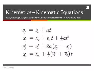
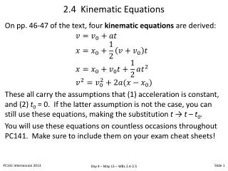
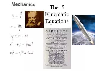
Summary of Equations • You will NOT be required to memorize these No Position No Time
The equation of the position vs. time graph is: The slope of this graph = velocity The y-intercept of this graph = initial position Lab Connection: Buggy Lab
The equation of the velocity-time graph is: The slope of this graph = acceleration The y-intercept of this graph = initial velocity Lab Connection: GIP’erLab
Equations that describe objects that change their velocities: Linear Graphs from Lab Equations from data General Equation X vs. t2 V vs. t V2 vs. X
Problem Solving Strategy • Show your work – ALWAYS! • Sketch of situation, motion map, x vs. t plot • Use three step method: • Equationin variable form (no numbers plugged in yet) • If necessary, show algebramid-steps (still no numbers) • Equation with value(s)for the variables (numbers!) • Finalanswer: boxed/circled with appropriate units and sig figs
Practice Problem #1 • A school bus is moving at 25 m/s when the driver steps on the brakes and brings the bus to a stop in 3.0 s. What is the average acceleration of the bus while braking? vf = vi = Δt = a = 0 m/s 25 m/s 3.0 s ? a= -8.3 m/s2
Practice Problem #2 • An airplane starts from rest and accelerates at a constant 3.00 m/s2 for 30.0 s before leaving the ground. (a) How far did it move? (b) How fast was it going when it took off? vf= vi= Δt = a = Δx= ? 0 m/s 30.0 s 3.00 m/s2 Δx= 1350 m ? v = 90.0 m/s