Download

1 / 59
640 likes | 713 Views
Modeling Species Distribution with MaxEnt. Bryce Maxell, Acting Director, Montana Natural Heritage Program & Scott Story, Nongame Data Manager, Montana Fish, Wildlife and Parks. Agenda - Wednesday. 8-9 Introduction to MaxEnt 9:05-10 Reptile and Amphibian Model Examples

E N D
Modeling Species Distribution with MaxEnt Bryce Maxell, Acting Director, Montana Natural Heritage Program & Scott Story, Nongame Data Manager, Montana Fish, Wildlife and Parks
Agenda - Wednesday • 8-9 Introduction to MaxEnt • 9:05-10 Reptile and Amphibian Model Examples • 10:05-11 Installation and Walkthrough of MaxEnt • 11:05-12 Preparation of Data • 12-1 Lunch • 1-1:55 Thresholds & Model Validation • 2-3 Using models in your DSS • 3 - 5 Hands-on Session • Tomorrow 8-11 Hands-on, Data Prep, Questions & Discussion
Installing and Running MaxEnt INSTALLATION
Download & Install • http://www.cs.princeton.edu/~schapire/maxent/ • Current MaxEnt Version = 3.3.3e • Requires Java Version 1.4 or later • Type java –version at command prompt • http://www.java.com • Extract the .zip file to a very simple directory • No spaces, no strange characters, short • C:\maxent • Three files are installed • Maxent.bat • Maxent.jar • Readme.txt • Download the tutorial Word document
Set PATH and customize .bat file • My Computer Properties Advanced Environment Variables System Variables PATH Edit • Add to end of the PATH ;c:\maxent • Change the maxent.bat file • Change the extension to .txt so that you can edit it with Notepad • Change line reading java -mx512m -jar maxent.jar to… • java -mx512m -jar c:\maxent\maxent.jar • Change the extension back to .bat • Note that changing the 512 to another number allocates more memory 512 Mb = 0.5 Gb 1024 = 1 Gb 1536 = 1.5 Gb 2048 = 2 Gb
Running MaxEnt Basic modeling run
Required Inputs • Species presence localities (“samples”) file • Environmental feature layers • Output directory
Change variable types as necessary Supply an output directory
What MaxEnt Does • Reads through each layer to • Determine type • Create .mxe file for each layer in maxent.cache • Extracts the random background and sample data • You will get warnings about points that are “missing some environmental data” • Calculates the gain until a threshold is reached • Creates the output grids for each species (this takes the longest) • Creates the thumbnail .png images
Time Required • Ten feature layers (3 categorical) • 46 million pixels • 2 Species • Intel Core 2 Quad CPU (2.83 GHz) • 4.00 GB RAM • Windows 7 • 32-bit Operating System • 512Mb of memory specified Without maxent.cache = 38 minutes With maxent.cache = 24 minutes
Running MaxEnt Examining output
Output • plots folder • logfile • maxentResults.csv • For each species • .asc • .html • .lambdas • _omission.csv • _sampleAverages.csv • _samplePredictions.csv
Logfile • Timestamp • Version of MaxEnt • Samples file name • Warnings • Command line to repeat • Species • Layers • Layertypes • Directories for: samples file, layers, output • Number of samples • Maximum gain
Gain • Closely related to deviance, a measure of GOF in GAM and GLM • Starts at zero and heads toward an asymptote • MaxEnt trying to come up with best fit • Average log probability of presence samples minus a constant • Gain indicates how closely the model is concentrated around presence samples • Avg likelihood of presence samples = exp(gain)
Gain Examples • McCown’s Longspur • Resulting gain: 2.275 • Average likelihood for presence points = 9.728 • Olive-sided Flycatcher • Resulting gain: 1.297 • Average likelihood for presence points = 3.658 • Average likelihood of the presence sample is X times higher than that of a background pixel
Html • Analysis of omission/commission • Receiver Operating Curve (AUC calculated) • Preset Thresholds • Pictures of the Model • Analysis of Variable Contributions • Raw Outputs
Sample Predictions File • Coordinates for all points • Test or Training • Predicted values • Raw • Cumulative • Logistic • Use this file to calculate deviance • Use samples procedure in ArcMap to extract the ones and zeros (above threshold or not)
Logistic Ouput High probability of suitable conditions Low predicted probability of suitable conditions White dots = training (1059 points or 75%) Purple dots = test (352 points or 25%)
Viewing Data in ArcMap • Build Raster Attribute Table (Categorical) • .vat.dbf • Build Histograms (Classified) • .aux • Build Pyramids • .rrd • .xml • For species output grids • Convert ASCII to Raster (Output Data Type = FLOATING) • Output as .bil (Band interleaved by line)
Running MaxEnt MORE Advanced parameters
Running MaxEnt Replicate runs
Running MaxEnt BATCH MODE
Preparation of Data Scott Story
Required Inputs • Species presence localities (“samples”) file • Environmental feature layers • Output directory
Getting Feature Data Ready • Same projection (coordinate system, units, datum) • Same resolution • Same extent • ESRI ascii format
Two Raster Datasets Land cover Precipitation Source = PRISM Climate Center Type = ASCII grid Cell size = 0.0083333333 Columns & Rows = 7025, 3105 Spatial Reference = undefined (see metadata) Pixel Type = Signed Integer (32-bit) • Source = Montana Natural Heritage Program • Type = IMAGINE Image • Cell size = 30 meters • Columns & Rows =33005, 24008 • Spatial Reference = Montana State Plane (NAD83) • Pixel Type = Unsigned Integer (8-bit)
Two Raster Datasets Land cover Precipitation
Making Rasters Match • Define coordinate systems for both • Set some environment variables • Tools Options Geoprocessing Tab Environments • General Settings: Extent and Snap Raster • Raster Analysis Settings: Cell Size, Mask • Project Raster • Select target raster to match for output cell size
Precipitation Reprojected & Resampled • Same exact extent • Same exact number or rows & columns • Same exact cell size • Real test is…does Maxent throw any errors? • In this case…it worked! • Getting all your data layers squared away will take some time!
Types of Environmental Features • Continuous (Quantitative) • Interval-scale (interval data, order, linear scale) • Ordinal variables (scale unknown-transformed?, rank clear) • Ratio-scale (interval data, ordered, not on linear scale, e. g. temp on F or C scale) • Categorical (Qualitative) • Nominal (e.g. gender) • Ordinal (has order, e.g. low to great) • Dummy variables from quantitative (classes) • Name the ASCII files with CONT or CAT prefix
Preparing Point Data • Create a separate file for each species • Combine them all\groups of them into one file • Probably want to retain a unique identifier • May want to setup scripts in ArcGIS to extract presence data • Might also want more control of how background data is selected • Let’s look at an example script - ExtractModelInputData.py
Other “Feature” Layers • Masks • useful if you want to train a model using only a subset of the region • mask.asc • containing a constant value (1, for example) in area of interest and no-data values everywhere else. • Bias • assumption that species occurrence data are unbiased • good understanding of the spatial pattern • values should indicate relative sampling effort
Representing the output THRESHOLDS