Download
1 / 9
140 likes | 744 Views
Trip Distribution Modeling Part III. CE 573 Transportation Planning Lecture 14. Objectives. Growth factoring Types of constraints Methods. Future. Now. Growth Factoring. Concept: X FUTURE = X NOW *(growth factor) Applications Beyond regional scope Gravity model inadequate

E N D
Trip Distribution Modeling Part III CE 573 Transportation Planning Lecture 14
Objectives • Growth factoring • Types of constraints • Methods Michael Dixon
Future Now Growth Factoring • Concept: • XFUTURE = XNOW*(growth factor) • Applications • Beyond regional scope • Gravity model inadequate • Too difficult to forecast independent variables Michael Dixon
Definitions and Constraints • The trip matrix total: T • Tij is the number of trips going from origin i to destination j. • TLDk is the number of trips in cost-bin k • Typical trip matrix constraints Michael Dixon
Growth Factor Methods • t = initial OD matrix • Uniform growth factorTij = τ*tij. • Singly constrained growth-factor methods OR Michael Dixon
Growth Factor Methods (cont.) • Doubly constrained growth factorshave growth factors for origins and destinations (), where… • instead of ai and bj being the growth factors for origin i and destination j, they are adjustments made to each O-D pair volume in order to achieve the target values Oi and Dj required by the growth factors for the origins and destinations Michael Dixon
Growth Factor Methods (cont.)—doubly constrained • BI-PROPORTIONAL ALGORITHM: • Step 1: Set bj to 1.0, determine initial trip matrix, and solve for ai that meet origin constraints, given the latest bj values. • Recalculate Tij with new ai values • Step 2: Solve for bj that meet the destinations constraints given the latest ai values and the previous bj values. • Recalculate Tij with new bj values and the latest ai values. • m-1 indicates previous iteration Michael Dixon
Growth Factor Methods (cont.)—doubly constrained • Step 3: Keeping the bj values fixed solve for ai that satisfy origin constraints given the ai from the last iteration (iteration m-1). • m-1 indicates previous iteration • Repeat steps 2 and 3 until changes in ai and bj are sufficiently small. • Note: This algorithm assumes that both sets of constraints can be satisfied simultaneously. In other words, the following must be true: Michael Dixon
Advantages and limitations of growth-factor methods • Advantages • simple • Disadvantages • requires an initial O-D matrix • no consideration given to changes in transport costs Michael Dixon