Download

1 / 36
360 likes | 367 Views
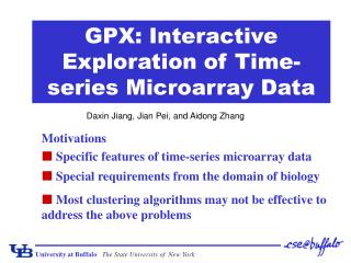
GPX: Interactive Exploration of Time-series Microarray Data. Daxin Jiang, Jian Pei, and Aidong Zhang. Motivations Specific features of time-series microarray data. Special requirements from the domain of biology. Most clustering algorithms may not be effective to address the above problems.

E N D
GPX: Interactive Exploration of Time-series Microarray Data Daxin Jiang, Jian Pei, and Aidong Zhang Motivations Specific features of time-series microarray data • Special requirements from the domain of biology • Most clustering algorithms may not be effective to address the above problems
Time-series Microarray Data Time 0 Time 1 Time 2 Gene expression levels are monitored at different time points during a time series.
Co-expressed Genes and Coherent Patterns Parallel coordinates for Iyer’s data Examples of co-expressed genes and coherent patterns in gene expression data • [1] Iyer, V.R. et al. The transcriptional program in the response of human fibroblasts to serum. Science, 283:83–87, 1999.
Example – Cell Cycle S phase Early G1 phase The cell cycle Expression patterns of cell-cycle regulated genes of yeast reported by Spellman et al. G2 phase Late G1 phase [2] Spellman et al., (1998). Comprehensive identification of cell cycle-regulated genes of the yeast Saccharomyces cerevisiae by microarray hybridization. Molecular Biology of the Cell 9, 3273-3297. M phase
Cluster Analysis • Partition the data set into several disjoint clusters • Each cluster is a group of co-expressed genes. • The centroid of the cluster is the coherent pattern. • Various of clustering methods • Partition-based approaches • Hierarchical approaches • Density-based approaches • ……
What the Data Look Like L. Zhang et al. Enhanced Visualization of Time Series through Higher Fourier Harmonics. BIOKDD 2003
High Connectivity of the Data ga gb Two genes with complete different patterns connected by a “bridge”
Hierarchies of Co-expressed Genes and Coherent Patterns The interpretation of co-expressed genes and coherent patterns mainly depends on the domain knowledge
To Split or Not • Dependent on “domain knowledge” group A1 group A2 group A
Which Split Option to Choose • Dependent on “domain knowledge” Various split options may correspond to different hypotheses regarding gene function.
What is a “Good” Clustering Algorithm • Form a hierarchical structure • Flexible and convenient to derive clusters • Support users’ domain knowledge • Handle the high connectivity effectively
Partition-based Approaches • Form a hierarchical structure? • Yes, if we use it as the split strategy in the divisive approach • Flexible and convenient to derive clusters? • No, since the parameters are hard to determine • Handle the high connectivity effectively? • No, since it partitions the data set by force
Cluster Borders Cut cluster borders by force
Hierarchical Approaches • Form a hierarchical structure? • Sure • Flexible and convenient to derive clusters? • Global threshold: convenient but not flexible • Handle the high connectivity effectively? • Depends on which inter-cluster measure is used • e.g., complete-link may be better than single-link
Density-based Approaches • Form a hierarchical structure? • Not explicitly • Possible if we adjust the parameters level by level • Flexible and convenient to derive clusters? • DBSCAN and DENCLUE use global thresholds • not flexible • OPTICS plots cluster structure • both flexible and convenient
Density-based Approaches • Handle the high connectivity effectively? • DBSCAN and OPTICS are not effective • “indirectly density-reachable” forms a chain • DENCLUE cuts the cluster border by force • center-defined clusters • a local maximum of density is the “center” of a cluster • other objects in the cluster are “attracted” to the local maximum
Our Solution– An Interactive Approach • Adopt a divisive approach to form a hierarchical structure • Users can choose whether to split or not • Still need one parameter • robust • easy to determine • Plot the cluster structure of the data set • Users can explore the data set by “drill down” and “roll up” operations based on their domain knowledge • Apply a novel strategy to handle the high connectivity. • Users can determine the cluster border
Genes Similarity gene g i1 0.99 gene g i2 0.98 gene g i3 0.98 gene g i4 0.95 gene g i5 0.94 gene g i6 0.94 … … … … gene g in-2 -0.44 gene g in-1 -0.45 gene g in -0.55 Pattern-based Strategy coherent pattern To find co-expressed genes and coherent expression patterns • Cluster-based strategy • First find clusters as co-expressed genes • Then use centroids as coherent expression patterns • Pattern-based strategy • First find coherent expression patterns • Then determine the co-expressed genes conforming to the pattern Pattern-based strategy
Distance Measure • Users are interested in overall shape • Euclidean distance does not work well • Normalize each data object O to O’ with a mean of 0 and a variance of 1 An object After normalization Shifting patterns m is the number of attributes, and are the mean and the standard deviation of O, respectively. Scaling patterns
Distance Measure • Similarity and Distance between two genes (objects) • The similarity and distance measure defined above are consistent • Given objects O1, O2, O3 and O4, Similarity(O1,O2)≥Similarity(O3,O4) if and only if Distance(O1,O2) Distance(O3,O4)
A Density-based Model • A group of co-expressed genes form a dense area; • Genes at the core area have high density, while genes at the boundary area have low density; • Genes at the boundary area are “attracted” towards the local maximum level by level.
Density Measures Radius-based density KNN-based density DENCLUE density
Definition of Density • We modify the density definition by Denclue[3] • The influence function (attraction function) • Given a data set D d(Oi,Oj) is the distance between Oi and Oj, and is a parameter is the estimated average similarity within a cluster • [3] Hinneburg, A. et al. An efficient approach to clustering in large multimedia database with noise. Proc. 4th Int. Con. on Knowledge discovery and data mining, 1998.
Attraction Tree • The “attractor” of object O is its nearest neighbor with a higher density than O. • Denoted by O Attractor(O). • We can derive an attraction tree based on the “attractor” relationship • The weight for each edge e(Oi,Oj) on the attraction tree is defined as the similarity between Oi and Oj. • Use Pearson’s correlation coefficient as similarity measure.
An Example of Attraction Tree An example data set The attraction tree • Three features of attraction tree: • self-closed: a group of objects conforming to the same coherent pattern forms an attraction subtree. • robust to intermediate genes (noise) • three levels of edge weights
Index List • Serialization of the attraction tree • Search the attraction tree based on the edge weight. • Order the genes in the “index list”. The attraction tree The index list
Index list Similarity curve for Iyer’sdata set
Coherent Pattern Index Graph • Compute the “coherent pattern index (CPI)” for each gene. p is a parameter, Sim(gi) is the similarity between gi and its parent gj on the attraction tree The index list The coherent pattern index graph
M phase S phase Early G1 phase Late G1 phase G2 phase
Validation Measure P1 C1 P2 C2 P3 C3 P4 C4 … … Pn Cm Ground truth patterns Reported patterns P1 is matched by C4 with similarity 0.95. (suppose Sim(P1,C4)=0.95) P2 is matched by C1 with similarity 0.90. (supposeSim(P2,C1)=0.9)
Comparison With Other Approaches The similarity between the pattern reported by different approaches and the corresponding pattern in the ground truth (if any)
Comparison with Optics Iyer’s data set Spellman’s data set
Effects of Parameters Spellman’s data set Iyer’s data set
Scalability • The algorithm scales well with large data sets. • The computation time is dominated by the distance calculation.