Download
1 / 103
1.03k likes | 1.23k Views
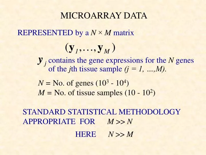
MICROARRAY DATA. REPRESENTED by a N × M matrix. contains the gene expressions for the N genes. of the j th tissue sample (j = 1, …,M). N = No. of genes (10 3 - 10 4 ) M = No. of tissue samples (10 - 10 2 ) . STANDARD STATISTICAL METHODOLOGY APPROPRIATE FOR M >> N.

E N D
MICROARRAY DATA REPRESENTED by a N ×Mmatrix contains the gene expressions for the N genes of the jth tissue sample (j = 1, …,M). N = No. of genes (103 - 104) M = No. of tissue samples (10 - 102) STANDARD STATISTICAL METHODOLOGY APPROPRIATE FORM >> N HERE N >> M
Microarray Data represented as N x M Matrix Sample 1 Sample 2 Sample M Gene 1 Gene 2 Gene N Expression Signature M columns (samples) ~ 102 N rows (genes) ~ 104 Expression Profile
Two Clustering Problems: • Clustering of genes on basis of tissues: genes not independent • Clustering of tissues on basis of genes: latter is a nonstandard problem in cluster analysis (n << p)
UNSUPERVISED CLASSIFICATION (CLUSTER ANALYSIS) INFER CLASS LABELSz1, …, zn of y1, …,yn Initially, hierarchical distance-based methods of cluster analysis were used to cluster the tissues and the genes Eisen, Spellman, Brown, & Botstein (1998, PNAS)
The notion of a cluster is not easy to define. There is a very large literature devoted to clustering when there is a metric known in advance; e.g. k-means. Usually, there is no a priori metric (or equivalently a user-defined distance matrix) for a cluster analysis. That is, the difficulty is that the shape of the clusters is not known until the clusters have been identified, and the clusters cannot be effectively identified unless the shapes are known.
In this case, one attractive feature of adopting mixture models with elliptically symmetric components such as the normal or t densities, is that the implied clustering is invariant under affine transformations of the data (that is, under operations relating to changes in location, scale, and rotation of the data). Thus the clustering process does not depend on irrelevant factors such as the units of measurement or the orientation of the clusters in space.
Hierarchical clustering methods for the analysis of gene expression data caught on like the hula hoop. I, for one, will be glad to see them fade. Gary Churchill (The Jackson Laboratory) Contribution to the discussion of the paper by Sebastiani, Gussoni, Kohane, and Ramoni. Statistical Science (2003) 18, 64-69.
Hierarchical (agglomerative) clustering algorithms are largely heuristically motivated and there exist a number of unresolved issues associated with their use, including how to determine the number of clusters. “in the absence of a well-grounded statistical model, it seems difficult to define what is meant by a ‘good’ clustering algorithm or the ‘right’ number of clusters.” (Yeung et al., 2001, Model-Based Clustering and Data Transformations for Gene Expression Data, Bioinformatics 17)
McLachlan and Khan (2004). On a resampling approach for tests on the number of clusters with mixture model-based clustering of the tissue samples. Special issue of the Journal of Multivariate Analysis 90 (2004) edited by Mark van der Laan and Sandrine Dudoit (UC Berkeley).
Attention is now turning towards a model-based approach to the analysis of microarray data For example: • Broet, Richarson, and Radvanyi (2002). Bayesian hierarchical model for identifying changes in gene expression from microarray experiments. Journal of Computational Biology9 • Ghosh and Chinnaiyan (2002). Mixture modelling of gene expression data from microarray experiments. Bioinformatics 18 • Liu, Zhang, Palumbo, and Lawrence(2003). Bayesian clustering with variable and transformation selection. In Bayesian Statistics 7 • Pan, Lin, and Le, 2002, Model-based cluster analysis of microarray gene expression data. Genome Biology 3 • Yeung et al., 2001, Model based clustering and data transformations for gene expression data, Bioinformatics 17
The notion of a cluster is not easy to define. There is a very large literature devoted to clustering when there is a metric known in advance; e.g. k-means. Usually, there is no a priori metric (or equivalently a user-defined distance matrix) for a cluster analysis. That is, the difficulty is that the shape of the clusters is not known until the clusters have been identified, and the clusters cannot be effectively identified unless the shapes are known.
In this case, one attractive feature of adopting mixture models with elliptically symmetric components such as the normal or t densities, is that the implied clustering is invariant under affine transformations of the data (that is, under operations relating to changes in location, scale, and rotation of the data). Thus the clustering process does not depend on irrelevant factors such as the units of measurement or the orientation of the clusters in space.
http://www.maths.uq.edu.au/~gjm McLachlan and Peel (2000), Finite Mixture Models. Wiley.
Mixture Software: EMMIX EMMIX for UNIX McLachlan, Peel, Adams, and Basford http://www.maths.uq.edu.au/~gjm/emmix/emmix.html
Basic Definition We letY1,…. Yndenote a random sample of sizenwhereYjis a p-dimensional random vector with probability density functionf (yj) where thef i(yj) are densities and thepiare nonnegative quantities that sum to one.
Mixture distributions are applied to data with two main purposes in mind: • To provide an appealing semiparametric framework in which to model unknown distributional shapes, as an alternative to, say, the kernel density method. • To use the mixture model to provide a model-based clustering. (In both situations, there is the question of how many components to include in the mixture.)
Shapes of Some Univariate Normal Mixtures Consider where denotes the univariate normal density with mean mand variance s2.
D=1 D=2 D=3 D=4 Figure 1: Plot of a mixture density of two univariate normalcomponents in equal proportions with common variance s2=1
D=1 D=2 D=3 D=4 Figure 2:Plot of a mixture density of two univariate normalcomponents in proportions 0.75 and 0.25 with common variance
Normal Mixtures • Computationally convenient for multivariate data • Provide an arbitrarily accurate estimate of the underlying density with g sufficiently large • Provide a probabilistic clustering of the data into g clusters - outright clustering by assigning a data point to the component to which it has the greatest posterior probability of belonging
where where constant constant MAHALANOBIS DISTANCE EUCLIDEAN DISTANCE MIXTURE OF g NORMAL COMPONENTS
k-means k-means SPHERICAL CLUSTERS MIXTURE OF g NORMAL COMPONENTS
With a mixture model-based approach to clustering, an observation is assigned outright to the ith cluster if its density in the ith component of the mixture distribution (weighted by the prior probability of that component) is greater than in the other (g-1) components.
Figure 7: Contours of the fitted component densities on the 2nd & 3rd variates for the blue crab data set.
Estimation of Mixture Distributions It was the publication of the seminal paper ofDempster, Laird, and Rubin (1977) on theEM algorithm that greatly stimulated interest inthe use of finite mixture distributions to model heterogeneous data. McLachlan and Krishnan (1997, Wiley)
If need be, the normal mixture model can be made less sensitive to outlying observations by using t component densities. • With this t mixture model-based approach, the normal distribution for each component in the mixture is embedded in a wider class of elliptically symmetric distributions with an additional parameter called the degrees of freedom.
The advantage of the t mixture model is that, although the number of outliers needed for breakdown is almost the same as with the normal mixture model, the outliers have to be much larger.
In exploring high-dimensional data sets for group structure, it is typical to rely on principal component analysis.
Two Groups in Two Dimensions. All cluster information would be lost by collapsing to the first principal component. The principal ellipses of the two groups are shown as solid curves.
Mixtures of Factor Analyzers A normal mixture model without restrictions on the component-covariance matrices may be viewed as too general for many situations in practice, in particular, with high dimensional data. One approach for reducing the number of parameters is to work in a lower dimensional space by using principal components; another is to use mixtures of factor analyzers (Ghahramani & Hinton, 1997).
Mixtures of Factor Analyzers Principal components or a single-factor analysis model provides only a global linear model. A global nonlinear approach by postulating a mixture of linear submodels
Biis ap x q matrix andDiis a diagonal matrix.
The Uj areiid N(O, Iq)independently of the errors ej, which areiidas N(O, D),where D is a diagonal matrix
Conditional onithcomponent membership of the mixture, whereUi1, ..., Uinareindependent, identically distibuted (iid)N(O, Iq),independently of theeij, which are iidN(O, Di),whereDiis a diagonal matrix(i = 1, ..., g).
An infinity of choices forBifor model still holds ifBi is replaced by BiCi whereCi is an orthogonal matrix. ChooseCi so that is diagonal Number of free parameters is then