Download

1 / 59
660 likes | 1.02k Views
Mining Time Series Data. CS240B Notes by Carlo Zaniolo UCLA CS Dept. With Slides from:. A Tutorial on Indexing and Mining Time Series Data ICDM '01 The 2001 IEEE International Conference on Data Mining November 29, San Jose Dr Eamonn Keogh

E N D
Mining Time Series Data CS240B Notes by Carlo Zaniolo UCLA CS Dept With Slides from: A Tutorial on Indexing and Mining Time Series Data ICDM '01The 2001 IEEE International Conference on Data Mining November 29, San Jose Dr Eamonn Keogh Computer Science & Engineering DepartmentUniversity of California - RiversideRiverside,CA 92521eamonn@cs.ucr.edu
Outline • Introduction, Motivation • Similarity Measures • Properties of distance measures • Preprocessing the data • Time warped measures • Indexing Time Series • Dimensionality reduction • Discrete Fourier Transform • Discrete Wavelet Transform • Singular Value Decomposition • Piecewise Linear Approximation • Symbolic Approximation • Piecewise Aggregate Approximation • Adaptive Piecewise Constant Approximation • Summary, Conclusions
What are Time Series? 29 28 27 26 25 24 23 0 50 100 150 200 250 300 350 400 450 500 25.1750 25.2250 25.2500 25.2500 25.2750 25.3250 25.3500 25.3500 25.4000 25.4000 25.3250 25.2250 25.2000 25.1750 .. .. 24.6250 24.6750 24.6750 24.6250 24.6250 24.6250 24.6750 24.7500 A time series is a collection of observations made sequentially in time. Note that virtually all similarity measurements, indexing and dimensionality reduction techniques discussed in this tutorial can be used with other data types.
Time Series are Ubiquitous! I • People measure things... • The presidents approval rating. • Their blood pressure. • The annual rainfall in Riverside. • The value of their Yahoo stock. • The number of web hits per second. • … and things change over time. Thus time series occur in virtually every medical, scientific and businesses domain.
Time Series are Ubiquitous! II A random sample of 4,000 graphics from 15 of the world’s newspapers published from 1974 to 1989 found that more than 75% of all graphics were time series (Tufte, 1983).
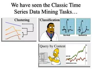
Classification Time Series Similarity Clustering Defining the similarity between two time series is at the heart of most time series data mining applications/tasks Rule Discovery 10 s = 0.5 c = 0.3 Thus time series similarity will be the primary focus of this tutorial. Query by Content Query Q (template)
Why is Working With Time Series so Difficult? Part I Answer: How do we work with very large databases? • 1 Hour of EKG data:1 Gigabyte. • Typical Weblog: 5 Gigabytes per week. • Space Shuttle Database: 158 Gigabytes and growing. • Macho Database: 2 Terabytes, updated with 3 gigabytes per day. Since most of the data lives on disk (or tape), we need a representation of the data we can efficiently manipulate.
Why is Working With Time Series so Difficult? Part II Answer: We are dealing with subjective notions of similarity. The definition of similarity depends on the user, the domain and the task at hand. We need to be able to handle this subjectivity.
Why is working with time series so difficult? Part III • Answer: Miscellaneous data handling problems. • Differing data formats. • Differing sampling rates. • Noise, missing values, etc.
Similarity Matching Problem: Flavors 1 1: Whole Matching Query Q (template) 6 1 7 2 8 3 C6is the best match. 9 4 10 5 Database C Given a Query Q, a reference database C and a distance measure, find the Cithat best matches Q.
Similarity matching problem: flavor 2 Query Q (template) 2: Subsequence Matching Database C The best matching subsection. Given a Query Q, a reference database C and a distance measure, find the location that best matches Q. Note that we can always convert subsequence matching to whole matching by sliding a window across the long sequence, and copying the window contents.
After all that background we might have forgotten what we are doing and why we care! So here is a simple motivator and review.. You go to the doctor because of chest pains. Your ECG looks strange… You doctor wants to search a database to find similar ECGS, in the hope that they will offer clues about your condition... • Two questions: • How do we define similar? • How do we search quickly?
Similarity is always subjective.(i.e. it depends on the application) • All models are wrong, but some are useful… This slide was taken from: A practical Time-Series Tutorial withMATLAB—presented at ECLM PAKDD 2005, by Michalis Vlachos.
Metric Euclidean Distance Correlation Triangle Inequality: d(x,z) ≤ d(x,y) + d(y,z) Assume: d(Q,bestMatch) = 20 and d(Q,B) =150 Then, since d(A,B)=20 d(Q,A) ≥ d(Q,B) – d(B,A) d(Q,A) ≥ 150 – 20 = 130 We do not need to get A from disk Non-Metric Time Warping LCSS: longest common sub-sequence Distance functions
Preprocessing the data before distance calculations • If we naively try to measure the distance between two “raw” time series, we may get very unintuitive results. • This is because Euclidean distance is very sensitive to some distortions in the data. For most problems these distortions are not meaningful, and thus we can and should remove them. • In the next 4 slides I will discuss the 4 most common distortions, and how to remove them. • Offset Translation • Amplitude Scaling • Linear Trend • Noise
3 3 2.5 2.5 2 2 1.5 1.5 1 1 0.5 0.5 0 0 0 50 100 150 200 250 300 0 50 100 150 200 250 300 0 50 100 150 200 250 300 Transformation I: Offset Translation D(Q,C) Q = Q - mean(Q) C = C - mean(C) D(Q,C) 0 50 100 150 200 250 300
0 100 200 300 400 500 600 700 800 900 1000 Transformation II: Amplitude Scaling 0 100 200 300 400 500 600 700 800 900 1000 Q = (Q - mean(Q)) / std(Q) C = (C - mean(C)) / std(C) D(Q,C)
5 4 3 2 12 1 10 0 8 -1 6 -2 4 -3 0 20 40 60 80 100 120 140 160 180 200 2 0 -2 5 -4 0 20 40 60 80 100 120 140 160 180 200 4 3 2 1 0 -1 -2 -3 0 20 40 60 80 100 120 140 160 180 200 Transformation III: Linear Trend After offset translation And amplitude scaling Removed linear trend The intuition behind removing linear trend is this. Fit the best fitting straight line to the time series, then subtract that line from the time series.
8 8 6 6 4 4 2 2 0 0 -2 -2 -4 -4 0 20 40 60 80 100 120 140 0 20 40 60 80 100 120 140 Transformation IIII: Noise Q = smooth(Q) C = smooth(C) The intuition behind removing noise is this. Average each datapoints value with its neighbors. D(Q,C)
A Quick Experiment to Demonstrate the Utility of Preprocessing the Data 3 Clustered using Euclidean distance on the raw data 2 9 6 8 5 7 4 1 Clustered using Euclidean distance on the raw data, after removing noise, linear trend, offset translation and amplitude scaling. 9 8 7 5 6 4 3 2 1
Summary of Preprocessing The “raw” time series may have distortions which we should remove before clustering, classification etc. Of course, sometimes the distortions are the most interesting thing about the data, the above is only a general rule. We should keep in mind these problems as we consider the high level representations of time series which we will encounter later (Fourier transforms, Wavelets etc). Since these representations often allow us to handle distortions in elegant ways.
Dynamic Time Warping Fixed Time Axis Sequences are aligned “one to one”. “Warped” Time Axis Nonlinear alignments are possible. Note: We will first see the utility of DTW, then see how it is calculated.
Sunday Friday Saturday Thursday Monday Tuesday Wednesday Utility of Dynamic Time Warping: Example II, Data Mining Power-Demand Time Series. Each sequence corresponds to a week’s demand for power in a Dutch research facility in 1997 [van Selow 1999]. Wednesday was a national holiday
Hierarchical clustering with Euclidean Distance. <Group Average Linkage> 4 5 3 6 The two 5-day weeks are correctly grouped. Note however, that the three 4-day weeks are not clustered together. Also, the two 3-day weeks are also not clustered together. 7 2 1
6 4 7 5 3 2 1 Hierarchical clustering with Dynamic Time Warping. <Group Average Linkage> The two 5-day weeks are correctly grouped. The three 4-day weeks are clustered together. The two 3-day weeks are also clustered together.
Dynamic Time-Warping • (how does it work?)The intuition is that we copy an element multiple times so as to achieve a better matching Euclidean distance: d = 1 T1 = [1, 1, 2, 2] | | | | T2 = [1, 2, 2, 2] Warping distance: d = 0 T1 = [1, 1, 2, 2] | | | T2 = [1, 2, 2, 2]
Q wk p j C w1 1 1 n i Computing the Dynamic Time Warp Distance I Note that the input sequences can be of different lengths Q |n| |p| C
Q wk p j C w1 1 1 n i Computing the Dynamic Time Warp Distance II Q |n| |p| C Every possible mapping from Q to C can be represented as a warping path in the search matrix. We simply want to find the cheapest one… Although there are exponentially many such paths, we can find one in only quadratic time using dynamic programming.
Complexity of Time Warping • Time taken to create hierarchical clustering of power-demand time series. • Time to create dendrogram • using Euclidean Distance 1.2 seconds • Time to create dendrogram • using Dynamic Time Warping 3.40 hours • How to speed it up. • Approach 1: Complexity is O(n2). We can reduce it to O(n) simply by restricting the warping path. • Approach 2: Approximate the time series with some compressed or downsampled representation, and do DTW on the new representation.
Fast Approximations to Dynamic Time Warp Distance II 22.7 sec 1.3 sec .. strong visual evidence to suggests it works well. Good experimental evidence the utility of the approach on clustering, classification and query by content problems also has been demonstrated.
Weighted Distance Measures I Intuition: For some queries different parts of the sequence are more important. Weighting features is a well known technique in the machine learning community to improve classification and the quality of clustering.
Relevance Feedback for Time Series The original query The weigh vector. Initially, all weighs are the same. Note: In this example we are using a piecewise linear approximation of the data. We will learn more about this representation later.
The initial query is executed, and the five best matches are shown (in the dendrogram) One by one the 5 best matching sequences will appear, and the user will rank them from between very bad (-3) to very good (+3)
Based on the user feedback, both the shape and the weigh vector of the query are changed. The new query can be executed. The hope is that the query shape and weights will converge to the optimal query. Two paper consider relevance feedback for time series. L Wu, C Faloutsos, K Sycara, T. Payne: FALCON: Feedback Adaptive Loop for Content-Based Retrieval. VLDB 2000: 297-306
Motivating Example Revisited... You go to the doctor because of chest pains. Your ECG looks strange… You doctor wants to search a database to find similar ECGS, in the hope that they will offer clues about your condition... • Two questions: • How do we define similar? • How do we search quickly?
Query Q Find shapes like this In this DB Indexing Time Series • We have seen techniques for assessing the similarity of two time series. • However we have not addressed the problem of finding the best match to a query in a large database... • We need someway to index the data... • A topics extensively discussed in topical literature that we will not discuss here for lack of time—also it might not be applicable to data streams
Compression – Dimensionality Reduction • Project all sequences into a new space, and search this space instead.
An Example of a Dimensionality Reduction Technique Raw Data 0.4995 0.5264 0.5523 0.5761 0.5973 0.6153 0.6301 0.6420 0.6515 0.6596 0.6672 0.6751 0.6843 0.6954 0.7086 0.7240 0.7412 0.7595 0.7780 0.7956 0.8115 0.8247 0.8345 0.8407 0.8431 0.8423 0.8387 … The graphic shows a time series with 128 points. The raw data used to produce the graphic is also reproduced as a column of numbers (just the first 30 or so points are shown). C 0 20 40 60 80 100 120 140 n = 128
Dimensionality Reduction (cont.) Fourier Coefficients Raw Data 1.5698 1.0485 0.7160 0.8406 0.3709 0.4670 0.2667 0.1928 0.1635 0.1602 0.0992 0.1282 0.1438 0.1416 0.1400 0.1412 0.1530 0.0795 0.1013 0.1150 0.1801 0.1082 0.0812 0.0347 0.0052 0.0017 0.0002 ... 0.4995 0.5264 0.5523 0.5761 0.5973 0.6153 0.6301 0.6420 0.6515 0.6596 0.6672 0.6751 0.6843 0.6954 0.7086 0.7240 0.7412 0.7595 0.7780 0.7956 0.8115 0.8247 0.8345 0.8407 0.8431 0.8423 0.8387 … We can decompose the data into 64 pure sine waves using the Discrete Fourier Transform (just the first few sine waves are shown). The Fourier Coefficients are reproduced as a column of numbers (just the first 30 or so coefficients are shown). Note that at this stage we have not done dimensionality reduction, we have merely changed the representation... C 0 20 40 60 80 100 120 140 . . . . . . . . . . . . . .
An Example of a Dimensionality Reduction Technique III Raw Data 0.4995 0.5264 0.5523 0.5761 0.5973 0.6153 0.6301 0.6420 0.6515 0.6596 0.6672 0.6751 0.6843 0.6954 0.7086 0.7240 0.7412 0.7595 0.7780 0.7956 0.8115 0.8247 0.8345 0.8407 0.8431 0.8423 0.8387 … Truncated Fourier Coefficients Fourier Coefficients 1.5698 1.0485 0.7160 0.8406 0.3709 0.4670 0.2667 0.1928 0.1635 0.1602 0.0992 0.1282 0.1438 0.1416 0.1400 0.1412 0.1530 0.0795 0.1013 0.1150 0.1801 0.1082 0.0812 0.0347 0.0052 0.0017 0.0002 ... 1.5698 1.0485 0.7160 0.8406 0.3709 0.4670 0.2667 0.1928 n = 128 N = 8 Cratio = 1/16 C C’ 0 20 40 60 80 100 120 140 … however, note that the first few sine waves tend to be the largest (equivalently, the magnitude of the Fourier coefficients tend to decrease as you move down the column). We can therefore truncate most of the small coefficients with little effect. We have discarded of the data.
An Example of a Dimensionality Reduction Technique IIII Fourier Coefficients Raw Data 1.5698 1.0485 0.7160 0.8406 0.3709 0.1670 0.4667 0.1928 0.1635 0.1302 0.0992 0.1282 0.2438 0.2316 0.1400 0.1412 0.1530 0.0795 0.1013 0.1150 0.1801 0.1082 0.0812 0.0347 0.0052 0.0017 0.0002 ... 0.4995 0.5264 0.5523 0.5761 0.5973 0.6153 0.6301 0.6420 0.6515 0.6596 0.6672 0.6751 0.6843 0.6954 0.7086 0.7240 0.7412 0.7595 0.7780 0.7956 0.8115 0.8247 0.8345 0.8407 0.8431 0.8423 0.8387 … Sorted Truncated Fourier Coefficients 1.5698 1.0485 0.7160 0.8406 0.2667 0.1928 0.1438 0.1416 C C’ 0 20 40 60 80 100 120 140 Instead of taking the first few coefficients, we could take the best coefficients This can help greatly in terms of approximation quality, but makes indexing hard (impossible?). Note this applies also to Wavelets
0 20 40 60 80 100 120 0 20 40 60 80 100 120 0 20 40 60 80 100 120 0 20 40 60 80 100 120 0 20 40 60 80 100 120 0 20 40 60 80 100 120 DFT DWT SVD APCA PAA PLA Morinaka, Yoshikawa, Amagasa, & Uemura, PAKDD 2001 Korn, Jagadish & Faloutsos. SIGMOD 1997 Chan & Fu.ICDE 1999 Agrawal, Faloutsos, &. Swami. FODO 1993 Faloutsos, Ranganathan, & Manolopoulos. SIGMOD 1994 Keogh, Chakrabarti, Pazzani & MehrotraSIGMOD 2001 Keogh, Chakrabarti, Pazzani & Mehrotra KAIS 2000 Yi & Faloutsos VLDB 2000 Compressed Representations
Discrete Fourier Transform I Basic Idea: Represent the time series as a linear combination of sines and cosines, but keep only the first n/2 coefficients. Why n/2 coefficients? Because each sine wave requires 2 numbers, for the phase (w) and amplitude (A,B). X X' 0 20 40 60 80 100 120 140 Jean Fourier 1768-1830 0 1 2 3 4 5 Excellent free Fourier Primer Hagit Shatkay, The Fourier Transform - a Primer'', Technical Report CS-95-37, Department of Computer Science, Brown University, 1995. http://www.ncbi.nlm.nih.gov/CBBresearch/Postdocs/Shatkay/ 6 7 8 9
Discrete Fourier Transform II • Pros and Cons of DFT as a time series representation. • Good ability to compress most natural signals. • Fast, off the shelf DFT algorithms exist. O(nlog(n)). • (Weakly) able to support time warped queries. • Difficult to deal with sequences of different lengths. • Cannot support weighted distance measures. X X' 0 20 40 60 80 100 120 140 0 1 2 3 4 5 6 Note: The related transform DCT, uses only cosine basis functions. It does not seem to offer any particular advantages over DFT. 7 8 9
X X' DWT 0 20 40 60 80 100 120 140 Haar 0 Haar 1 Haar 2 Haar 3 Haar 4 Haar 5 Haar 6 Haar 7 Discrete Wavelet Transform I Basic Idea: Represent the time series as a linear combination of Wavelet basis functions, but keep only the first N coefficients. Although there are many different types of wavelets, researchers in time series mining/indexing generally use Haar wavelets. Haar wavelets seem to be as powerful as the other wavelets for most problems and are very easy to code. Alfred Haar 1885-1933 Excellent free Wavelets Primer Stollnitz, E., DeRose, T., & Salesin, D. (1995). Wavelets for computer graphics A primer: IEEE Computer Graphics and Applications.
X = {8, 4, 1, 3} h1= 4 = mean(8,4,1,3) h2 = 2 = mean(8,4) - h1 h3 = 2 = (8-4)/2 h4 = -1 = (1-3)/2 8 7 6 5 4 3 2 1 I have converted a raw time series X ={8, 4, 1, 3}, into the Haar Wavelet representation H = [4, 2 , 2, 1] We can covert the Haar representation back to raw signal with no loss of information... h1 = 4 h2 = 2 h3 = 2 h4 = -1 X = {8, 4, 1, 3} 8 7 6 5 4 3 2 1
X X' DWT 0 20 40 60 80 100 120 140 Haar 0 Haar 1 Haar 2 Haar 3 Haar 4 Haar 5 Haar 6 Haar 7 Discrete Wavelet Transform III • Pros and Cons of Wavelets as a time series representation. • Good ability to compress stationary signals. • Fast linear time algorithms for DWT exist. • Able to support some interesting non-Euclidean similarity measures. • Works best if N is = 2some_integer. Otherwise wavelets approximate the left side of signal at the expense of the right side. • Cannot support weighted distance measures. Open Question: We have only considered one type of wavelet, there are many others. Are the other wavelets better for indexing? YES: I. Popivanov, R. Miller. Similarity Search Over Time Series Data Using Wavelets. ICDE 2002. NO: K. Chan and A. Fu. Efficient Time Series Matching by Wavelets. ICDE 1999 Obviously, this question still open...
eigenwave 0 eigenwave 1 eigenwave 2 eigenwave 3 eigenwave 4 eigenwave 5 eigenwave 6 eigenwave 7 Singular Value Decomposition Basic Idea: Represent the time series as a linear combination of eigenwaves but keep only the first N coefficients. SVD is similar to Fourier and Wavelet approaches is that we represent the data in terms of a linear combination of shapes (in this case eigenwaves). SVD differs in that the eigenwaves are data dependent. SVD has been successfully used in the text processing community (where it is known as Latent Symantec Indexing ) for many years—but it is computationally expensive Good free SVD Primer Singular Value Decomposition - A Primer. Sonia Leach X X' SVD James Joseph Sylvester 1814-1897 0 20 40 60 80 100 120 140 Camille Jordan (1838--1921) Eugenio Beltrami 1835-1899
eigenwave 0 eigenwave 1 eigenwave 2 eigenwave 3 eigenwave 4 eigenwave 5 eigenwave 6 eigenwave 7 Singular Value Decomposition (cont.) How do we create the eigenwaves? We have previously seen that we can regard time series as points in high dimensional space. We can rotate the axes such that axis 1 is aligned with the direction of maximum variance, axis 2 is aligned with the direction of maximum variance orthogonal to axis 1 etc. Since the first few eigenwaves contain most of the variance of the signal, the rest can be truncated with little loss. X X' SVD 0 20 40 60 80 100 120 140
Piecewise Linear Approximation I Basic Idea: Represent the time series as a sequence of straight lines. Lines could be connected, in which case we are allowed N/2 lines If lines are disconnected, we are allowed only N/3 lines Personal experience on dozens of datasets suggest disconnected is better. Also only disconnected allows a lower bounding Euclidean approximation X Karl Friedrich Gauss 1777 - 1855 X' 0 20 40 60 80 100 120 140 • Each line segment has • length • left_height • (right_height can be inferred by looking at the next segment) • Each line segment has • length • left_height • right_height